Journal of Stock & Forex Trading
Open Access

Panel VAR Model Applied to Foreign Trade between Portugal and Regional Economic Blocs

Nerhum Laurindo Sandambi^{* *}Correspondence: Nerhum Laurindo Sandambi, Department of Economics, University of Aveiro, Lisbon, Portugal, Email:

Author info »

Introduction

The growth of Portuguese foreign trade began in the 20^th century, with the opening up of the economy, the development of industry and a marked diversification of goods for export. The commitment to industrialization began above all in the 1960's, driven by imports of investment goods from developed countries (mostly from the countries that make up the current European Union). For many years, Portugal's foreign trade was marked by a strong balance of payments deficit (even after joining the European Community bloc), associated with this deficit is the continuous import of goods and services. Exports at the time were mainly covered by wine, but products such as footwear and clothing made up the diversification mix, as well as other products that emerged as a result of the diversification of exports at the time and some agricultural products. Despite the low level of qualification, substantial gains in added value were made when footwear, clothing and other industrial products began to be exported instead of bulk wine and other food products. These gains are mainly reflected in the evolution of the terms of trade [1].

The main destination for Portuguese exports has always been the European Union (EU) countries, especially Spain, Germany and France, which account for 21.70 percent, 11.10 per ent and 13.40 percent respectively.

Portugal's entry into the European community bloc has strengthened existing bilateral economic relations and has had a major impact on the Portuguese economy. The main impacts on the Portuguese economy following its accession to the European Economic Community (EEC) are analysed below. Where three periods are considered the period immediately following accession, in which the impact was clearly positive, allowing the Portuguese economy to grow at a relatively high rate; the period of preparation for the single currency, in which external competitiveness problems arose due to the macroeconomic policy followed and the changes in world trade; and finally the period from the creation of the single currency to the present day, in which the Portuguese economy has fallen into crisis and in which the high level of indebtedness strongly conditions the possibilities for future growth, I concluded [2].

In recent years, Portugal's trade balance has shown continuous improvements, which on the one hand were due to the financial bailout requested from the IMF and ECB and on the other hand, the growth in diversified exports and the increase in the level of output, mainly driven by substantial improvements in the industrial sector and a strong presence of foreign capital investments in the country. Also noteworthy is the expansion of exports to markets such as the United States of America, which is considered to be the largest destination for Portuguese exports in extra-EU trade, accounting for 5.5 percent of exports in 2017, according to data from the European Commission. However, panel VAR models try to capture the impact of explanatory variables through Impulse Response Functions (IRF). Love and Zicchino analyse the dynamic relationships between the financial conditions of companies and investments for a set of 36 countries, using Impulse response functions and show that the impact of financial factors on investments, which indicates financing restrictions, is significantly greater in countries with a less developed financial system. The authors also call for the role of financial development in improving the allocation and growth of capital, they conclude [3].

Grossmann, et al., analysing the dynamics of global exchange rate volatility for 29 economies using impulse response functions, show how shocks to the high-frequency and low-frequency components of volatility differ. According to the authors, using a conventional temporal approach to study volatility can lead to spurious results. The main results of the study show that the feedback effects of exchange rate volatility on macroeconomic and financial variables are found to be much stronger for developing countries than for developed economies. These results are confirmed by variance decompositions and are largely immune to various robustness checks. Trung analyses the collateral effects of uncertainty shocks from the United States of America (USA) on emerging economies, the authors' results show that uncertainty shocks from the USA are risks and therefore abandon the inflow of capital, investment, consumption, exports and production from emerging economies. This translates into a depreciation of emerging market currencies. As a result, according to the findings, a fall in the short-term interest rate of emerging economies is predicted in order to react to US uncertainty shocks. The authors' conclusions help in part to explain the slow recovery of the world economy after the global financial crisis of 2008-2009. Jacobs, et al., study the causal relationship between public debt ratios and economic growth rates for 31 EU and OECD countries, the authors estimated a panel VAR model that incorporates the long-term real interest rate on government bonds as a vehicle for transmitting shocks to both the public debt-to-GDP ratio and the economic growth rate, the results do not show a causal link between public debt and growth regardless of the levels of the public debt ratio. On the contrary, the authors found a causal relationship between growth and public debt. In countries with high debts, the negative impact of growth on public debt is reinforced by an increase in the longterm real interest rate, which in turn decreases interest-sensitive demand and leads to a further increase in the public debt ratio [4].

Aslan, et al., explores the impacts of the real effective exchange rate on international trade, using quarterly data from 2005:Q1-2018:Q4, the results do not accurately show whether real exchange rate shocks affect export volumes in emerging markets, export volume responses to real exchange rate shocks are heterogeneous across countries, with commodity-exporting countries, on average, having a lower export response to real exchange rate movements. Furthermore, the authors found that although the magnitude of the response of export volumes to exchange rate shocks is positively related to exchange rate volatility, the higher rate of export market penetration helps insulate the economy from real exchange rate shocks. Overall, the results have broad policy implications indicating that policymakers need to pay attention to their countries' exchange rate volatility and expand their export competition in world trade, the authors conclude. Arvin, et al., analyse the impact of stock market development on inflation and economic growth in 16 Asian countries from 1988-2012. Using Granger causality tests, the results show that there is a long-term relationship between the variables analysed. Morteza, et al., study the effects of oil price shocks on technology transfer in OPEC members, the results show that oil price shocks have a positive effect on capital, imports of intermediate goods and FDI, while R and D expenditure was reduced. In addition, the convergence of the models was proven by VECM analysis and the long-term relationship. Finally, the coefficient between capital, imports of intermediate goods and FDI leads to the fact that imports without FDI make the model divergent, which means that the transfer of knowledge and management is highly valued in the technology transfer process and is possible with the use of FDI; the authors conclude [5].

Behaviour of foreign trade between Portugal and the countries under review

Portugal maintains a perfect bilateral relationship with its partners, especially those that are considered to be strategic allies and have a huge importance in economic relations, so in recent years foreign trade with the main partners has shown significant improvements, both in terms of the trade balance and in terms of export flows, with emphasis on relations with the European union economic bloc, which accounts for 74% of foreign trade, according to INE data. With regard to other partners such as the UK, which is of great significance to Portugal, relations have been stable and favourable in recent years, with the trade balance between these two countries being significantly stable, despite the "Grexit". From January to September 2017, 7.9% of exports and 4.3% of imports of Portuguese goods and services went to the British market. The USA is Portugal's biggest economic partner outside the EU, accounting for around 5% of Portuguese exports and a favourable trade balance. Given its economic size, China is a major market for Portugal, especially as a supplier and a major investor and the share of capital coming from China in large Portuguese companies should be emphasised. As far as Portuguese-speaking economic partners are concerned, the PALOP group represents an extremely important market as clients, while Brazil stands out as a very important partner for the Portuguese economy. The trade balance between Portugal and Brazil is positive, with an emphasis on exports of goods and services. Russia and South Africa are no less important, both with a positive trade balance. Figures 1 and 2 shows, interactively and explicitly, the foreign trade between Portugal and the regional blocs under analysis (Figures 1 and 2) [6].

Figure 1: Export structure.

Figure 2: Exports.

The graph in Figure 2 shows Portugal's exports with its partners for the periods analyzed, where we can see a marked increase in Portuguese exports to the European union, which is the largest destination for Portuguese exports, followed by the Kingdom, in line with the data from our analysis of Portuguese foreign trade with partners by regional bloc [7].

Materials and Methods

However, the section analyses the data and the methodology of the panel VAR model, the unit root tests and the cointegration tests.

Data

The data used in this analysis was mostly collected from international institutions such as the World Bank, IMF, COMESA and some statistical portals, Tables 1 and 2 show the data and its source and the descriptive statistics for the two models are shown in Tables 3 and 4 [8].

Table 1: Variables.

Table 2: Descriptive statistics.

VAR models were first introduced to the literature in Sims, in these models, the variables are taken as endogenous, for specific approaches with panel data, the models began to be analysed in Eakin, et al., where they estimate the model by equating instrumental variables to quasi-differentiated variables in the model and applying the GMM method, which produces consistent and efficient results [9].

The panel VAR model proposed by the authors has the following algebraic specification:

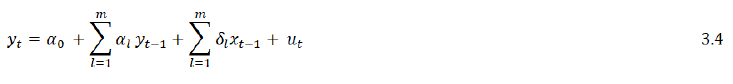
Where:

α e δ´s, are the linear projection coefficients of y_t, on the constant and past values of y_t e xt, m represents the lags, uit is the error term. It is assumed from the outset that the lags in the model must be the same for the y e x, the main drawback of these models is that they require many observations for the dependent and independent variables. For this study, we propose analysing the following model, according to the specification seen above [10].

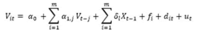
V_it, is the dependent variable;

X_t-1, is a vector that represents a set of explanatory variables in the model, whose representation is as follows:

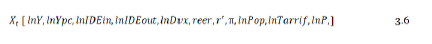
i, represents the countries being analysed, i(=1,….7), for Portugaleconomies under analysis;

Y, represents GDP;

Ypc, é o PIB per capita;

IDEin, is the foreign direct investment of the PALOP in Portugal;

IDEout, is Portugal's foreign direct investment in PALOP countries;

Dvx, is the external debt in millions of dollars;

reer, é is the real effective rate;

r', represents the real interest rate;

π, is the inflation rate;

Pop, is the population;

Tarrif, represents the average tariff applied to imported products;

P, is the price of oil;

f_i, are the unobserved individual effects;

t, represents the period under analysis, t=1980…2018;

u_t, represents the idiosyncratic error term;

The model is estimated using GMM methods, which take into account the mismatches with the model's instruments [11].

Unit root tests

Unit root tests are important when analysing time series or panel data, as they help to prevent spurious estimations when the series has unit roots. In this study we used the unit root tests analysed in Levin, et al., the test consists of carrying out separate Augmented Dickey-Fuller (ADF) regressions for each cross-section. The other step is to estimate the ratio of long-term to short-term standard deviations. The null hypothesis of the test specifies the presence of unit roots in each panel. However, there are other tests for unit roots in panels, analysed in Harris, et al., studies panels with display dimension N and T for infinity, other similar studies are analysed [12].

Cointegration tests

The relationship between the variables is analysed using cointegration tests. Test is based on Dickey Fuller and Augmented Dickey Fuler (ADF) estimated using the residuals of the fixed effects, the null hypothesis is that the series are not cointegrated under the alternative hypothesis that there is cointegration between the series.

Results

This chapter is dedicated to analysing and discussing the results; however, the results of the unit root tests, the cointegration tests, the impulse response functions and the results in general will be analysed. The correlation between the variables was analysed using the correlation matrices in the model, which can be found (Tables 3-5) [13].

Table 3: Results.

Table 4: Tests results.

Table 5: Results.

For the Westerlund Cointegration test, we had a P-value of 0.0000, verifying cointegration between the variables in the model. The same results can be seen in Table 5, where most of the results indicate the existence of cointegration between the variables in the model, thus demonstrating the long-term equilibrium between the variables (Figures 3-6) [14].

The results of the unit root tests in Table 3 indicate the presence of unit roots in the model, with the null hypothesis not being rejected. To solve the problem, first differences were applied and the results can be seen in Table 4, with the series without unit roots (Table 6) [15].

Table 6: Results.

Figure 3: Impulse response function results.

Figure 4: Impulse response functions.

Figure 5: Impulse response functions.

Figure 6: Impulse response function.

Discussion

This section presents the results of the estimations of the Panel VAR model, which was estimated using the GMM method. The coefficients show statistically significant results in the model. The analysis of the results will be reinforced with the impulse response functions, which allow us to obtain the impacts that one variable has on another, taking into account the structural shocks coming from different markets.

Figures 5 and 6 show the impact that the explanatory variables have on the trade volume variable, where we see the impact of foreign debt on foreign trade volume, the results show a negative impact that decreases until the 7^th period, this result is associated with the high levels of indebtedness that the countries under analysis have, countries such as the USA, Brazil and some countries that make up the European community bloc.

The tariff variable shows a continuous decrease, which may be due to the other variable remains stable, i.e., it changes little with structural shocks in the international market, i.e., when analysing the 10-year period. In general terms, the results do not differ much from those found in with the exception of the oil price and tariff variables, which do not affect foreign trade flows.

Conclusion

The study analysed foreign trade between Portugal and the regional economic blocs, respectively, the evidence for the European Union, United Kingdom, Brazil, South Africa, PALOP, Russia and China.

The study was carried out by estimating the dynamic panel VAR model, where we had the following results the GDP variables, being a measure of the economy, are statistically significant in the model and the results show that a 1% variation in GDP stimulates growth in trade. All other things being equal.

As for the real effective exchange rate variable, the results show that this does not affect the levels of trade flows between Portugal and the PALOP countries. These results can be verified with the Impulse Response Functions for the two periods under analysis. This result is associated with the fact that foreign trade is carried out on a large scale with countries that belong to the same EU economic bloc, given the standardisation of exchange rate policy and it also has to do with the fact that the euro is, for example, less devalued against the dollar, the yuan and the real.

Through the impulse response functions, the results show that trade policy through tariffs does not affect foreign trade between Portugal and the regional blocs. These results may be associated with the low tariff rates applied to trade between Portugal and the EU.

On the other hand, the foreign direct investment flows variables show that there is a certain influence on the levels of foreign trade flows between Portugal and the regional blocs. These results are related to the presence of capital from China and Brazil, for example. In general terms, the results are able to explain economic theory.

The levels of foreign direct investment, however, show a negative impact. This impact, however, is related to the reduction in Portuguese investment flows in the economies analysed. Income levels seem plausible, so a significant increase in income levels in third economies shows an increase in consumption and the need for the country to be able to increase imports, so the results seem plausible and capable of increasing foreign trade flows between the countries analysed.

Availability of Data and Materials

Available if required.

Competing Interests

Not applicable.

Funding

Not applicable.

Author Contributions

Formal, investigation.

Acknowledgements

I thank all the professors of the Economics department of the University of Evora.

Author information

Nerhum Laurindo Sandambi, holds a master's degree in economics from the University of Evora. Collaborator of CEFAGE-Centre for Advanced Training Studies in Management and Economics at the University of Evora.

References

1. Anderson JE. A theoretical foundation for the gravity equation. Am Econ Rev. 1979;69(1):106-116.

   [Google Scholar]

2. Arellano M, Bover O. Another look at the instrumental variable estimation of error-components models. J Econom. 1995;68(1):29-51.

   [Crossref] [Google Scholar]

3. Pradhan RP, Arvin MB, Samadhan B, Taneja S. The impact of stock market development on inflation and economic growth of 16 Asian countries: A Panel VAR approach. Appl Econom Int Dev. 2013;13(1):203-220.

   [Google Scholar]

4. Aslan C, Cepni O, Gul S. The impact of real exchange rate on international trade: Evidence from panel structural VAR model. J Int Trade Econ Dev. 2021;30(6):829-842.

   [Crossref] [Google Scholar]

5. Bergstrand JH. The gravity equation in international trade: Some microeconomic foundations and empirical evidence. Rev Econ Stat. 1985:474-481.

   [Crossref] [Google Scholar]

6. Boughanmi H. The trade potential of the Arab Gulf Cooperation Countries (GCC): A gravity model approach. J Econ Integr. 2008:42-56.

   [Google Scholar]

7. Breitung J, Meyer W. Testing for unit roots in panel data: Are wages on different bargaining levels cointegrated? Appl Econ. 1994;26(4):353-361.

   [Crossref] [Google Scholar]

8. Carrillo-Tudela C, Li CA. Trade blocks and the gravity model: Evidence from Latin American countries. J Econ Integr. 2004:667-689.

   [Google Scholar]

9. Holtz-Eakin D, Newey W, Rosen HS. Estimating vector autoregressions with panel data. Econometrica J Econom. 1988:1371-1395.

   [Crossref] [Google Scholar]

10. García EC, Navarro Pabsdorf M, Gomez Herrera E. The gravity model analysis: an application on MERCOSUR trade flows. J Econ Policy Reform. 2013;16(4):336-348.

    [Crossref] [Google Scholar]

11. Grossmann A, Love I, Orlov AG. The dynamics of exchange rate volatility: A panel VAR approach. J Int Financ Mark Inst Money. 2014;33:1-27.

    [Crossref] [Google Scholar]

12. Harris RD, Tzavalis E. Inference for unit roots in dynamic panels where the time dimension is fixed. J Econom. 1999;91(2):201-226.

    [Crossref] [Google Scholar]

13. Hausman JA. Specification tests in econometrics. Econom J Econom.1251-1271.

    [Crossref] [Google Scholar]

14. Im KS, Pesaran MH, Shin Y. Testing for unit roots in heterogeneous panels. J Econom. 2003;115(1):53-74.

    [Crossref] [Google Scholar]

15. Jacobs J, Ogawa K, Sterken E, Tokutsu I. Public debt, economic growth and the real interest rate: A panel VAR approach to EU and OECD countries. Appl Econ. 2020;52(12):1377-1394.

    [Crossref] [Google Scholar]