Human perception is the process of acquiring, interpreting, selecting and organizing sensory information to effectively interact with the environment. It is argued that the ability to perceive and direct visual attention to an object that warrants more detailed analysis is the most important of the senses. The oculomotor system has evolved to serve this purpose and, consequently, has important communicative value for studying neuromuscular integration.

Research involving sensorimotor control seeks to answer the fundamental question: How does our brain select inputs to produce a desired intention and manifest it in the form of movement. The difficulty associated with this question becomes more apparent for multi-body, multi-dimensional systems whose equations of motion are nonlinear and coupled. Since the eye is confined to three rotational degrees of freedom, and because the actions of its extraocular muscles are direct, the oculomotor system provides an initial context for gaining insight into more complex strategies of sensorimotor control.

Although extensive studies of eye movements have been useful for understanding the mechanisms of sensorimotor control, new findings associated with the mechanical characteristics of the ocular plant and neurological processing at much deeper levels have given rise to spirited debates questioning the brain’s role [1-4]. In other words, how much of the observed behavior of eye movements is a consequence of orbital mechanics and how much is due to neural processing. This is a recurring theme in the literature and deserves more attention.

Smooth pursuit eye movements

Through centuries of evolution, humans and primates have developed the sophisticated ability to track an object of interest with zero latency and in the presence of large neural transmission delays of up to 150 ms [5-7]. Once a moving target has been acquired, our eye begins to purse that target to maintain the object’s focus on a small region of the retina (Φ1.2 mm) called the fovea [8]. This region is packed with high threshold and color sensitive photoreceptors which allow us to view an image, in color and with high resolution.

A smooth pursuit is characterized as a slow eye movement with a maximum velocity of approximately 70°/s. It is commonly preceded by a fast eye movement called a saccade which is described as a ballistic repositioning of the gaze direction to that of a newly predicted target location as shown in Figure 1 [7,9,10].

Figure 1: Smooth pursuit of various ramp trajectories.

Effects of neural transmission delays

Time delays are a distinctive feature of biological information transmission and constitute the major difference between sensorimotor control and the modern control of mechatronic systems (see Table 1). Neural transmission delays severely limit the maximum gain that may be used if stability is to be maintained in closed loop feedback control [11-14]. Frequency domain modeling and analysis shows that time delays reduce the phase margin, which in turn lessens the damping ratio for the closed loop system and results in a response that is more oscillatory. The reduction in the phase also decreases the gain margin frequency and, hence, the admissible gain, thereby moving the system closer to instability [15-17].

System Type	Communication	Feedback Loop Delay	Actuator Bandwidth
Biological	Neurons 100 m/s	Trans-cortical>100 ms	Muscle << 10 Hz
Mechatronic	Electrons 108 m/s	Encoder/Tachometer<1 ms GPS 130 ms	Electro-magnetic>100 Hz Electro-hydraulic >> 1000 Hz

Table 1: Comparison of system operating variables for biological and mechatronic systems.

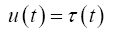
Consider the delayed position feedback control of a second order system (shown in Figure 2) that is used to describe the mechanical characteristics of the ocular plant (please refer to the methods section for more information regarding this model).

Figure 2: Destabilizing effects of time delay A) Westheimer model with position feedback delay. B) System response to an oscillatory input for three small time delays which are well below that of a neural transmission delay.

The response clearly illustrates how small delays in position feedback dramatically affect the stability of the system. What is more revealing is that their magnitudes are smaller than the delays observed in experimental recordings [18,19]. A clue as to how the sensorimotor system may overcome this challenge lies in the fact that muscle acts as a neuromuscular-actuator with non-zero output mechanical impedance [20-22]. Unlike a direct current, permanent magnet motor (DCPMM), which is meticulously designed to generate torque independent of displacement and velocity, muscle generates movement based on its length-tension and force-velocity characteristics [9,23,24]. The output mechanical impedance of muscle may provide many effects similar to feedback action without being vulnerable to the destabilizing effects of neural transmission delays [25-27].

Optimal control strategies in sensorimotor control

A mechatronic system can perform simple repetitive tasks faster and far more precisely than a human. Their actuator torque output is produced reliably every time based on a controlled input. The transmission lines through which the controller communicates with its sensors and transducers work a million times faster than our sensorimotor system and are not at the mercy of the destabilizing effects of time delays. Yet the paradox is that humans are far more dexterous and can adapt to their environment far better. So how do we, as engineers, model a highly variable biological system with these limitations? Here we turn to the powerful tools of optimal control theory which seek to determine the control signals that will cause a process to satisfy the physical constraints of a dynamic system and, at the same time, extremize a performance criteria or cost-to-go function [17,28].

Early adopters open loop optimization

Pioneering work done in the mid-1980s embodies the successful implementation of optimal control theory to study sensorimotor control. At this time Enderle et al. presented a time-optimal control model of saccadic eye movements [29,30]. This model accurately computes the separately maintained controls used to generate the active-state forces developed within the agonist and antagonist muscles. Moreover, the calculated controls have a direct correlation to the burst firing frequency of oculomotor nuclei in the midbrain which are experimentally verified. Although the development of this model began in the 1980s, its recent acceptance has been more pronounced as more researchers are turning to the principles of optimality to better understand the strategies used in sensorimotor control [12,31,32]. Enderle’s time-optimal control model continues to grow in popularity as it evolves, incorporating better parameter estimates [33,34] and adopting complete muscle fiber models [23,35- 37] Not only is the model being used to successfully test both visual and auditory stimulated saccades,18 but it has also been extended to describe complex three dimensional movements of the eyes relative to the head-neck complex [38,39].

An important note to be made regarding Enderle’s model is that it specifies a discrete point to point task and utilizes open-loop optimization. A stationary target is specified and the machinery of optimization generates the controls and movement profiles based on the performance criteria and the dynamic constraints inherent to the system. Because of the type of task and optimal control construct, this model does not need to address the destabilizing effects of neural transmission delay.

Closed loop optimization using sensory feedback

The time-optimal control model works perfectly for its intended purpose of acquiring a stationary target in minimum time, but what happens when we need to track a moving target and have to wrestle with the physiological limitations of neural transmission delays.

The work presented here aims to shed some light on that subject. Specifically, a linear quadratic tracking algorithm has been developed to smoothly pursue a target with a positional feedback delay of 150 ms. Optimization theory is used to construct a performance criterion that penalizes a weighted sum of the difference between the desired and actual state trajectory and the weighted sum of control effort, all of which is constrained by the dynamics of a simple second order model of the ocular plant. This is the first time that a linear system plant with realistic time delays has been presented in the literature.

Dynamic formulation

In 1954, Westheimer modeled horizontal saccades using a second order model of the ocular plant (Figure 3 adapted from Ref. [7]).

Figure 3: Second order eye dynamics A) Westheimer model of the ocular plant. The parameters J,B and K are rotational elements for moment of inertia, friction, and stiffness, respectively, and represent the eyeball and its associated viscoelasticity. The torque, t(t), applied to the eyeball is the result of antagonist muscle co-activation. The angular position of the eye is given by ?(t). B) Bond Graph of the model illustrating the respective energy flow in the system.

The differential equation governing the model is

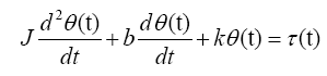   (1)

Or in standard second order form

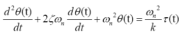   (2)

The transfer function for this model is simply

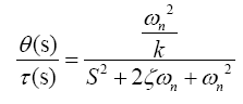   (3)

State-Space representation

Using the bond graph in Figure 3B and choosing Lagrangian state variables (i.e., Inertance flows, fi and displacements, qi) the respective state vector and control vector is defined as

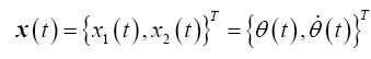   (4)
   (5)

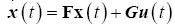
In state-space form

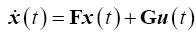   (6)
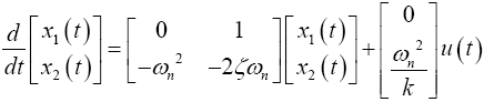   (7)

For a 20° target saccade, Westheimer’s reported the natural frequency and the damping ratio of the system to be ?_n² =120 rad/s and ?=1/v2 for an eye with a weight of 25 g and a radius of 11 mm. Converting to SI units of kg-N-m and solving for the stiffness (k=0.998), the stability matrix, F, and the control-effect matrix, G, can be represented numerically such that

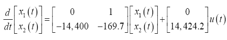   (8)

Tracking controller

The goal of the tracking problem is to maintain the system state x(t) as close as possible to the desired state (or reference trajectory) x_d(t) while using minimal control effort in the time interval, t?{t0, tf } [17,28]. The optimal control problem is therefore posed the following way:

Find the optimal control u*(t), for the state-space system given in (7) that tracks a desired trajectory, x_d(t) and minimizes the performance criteria

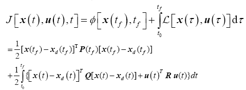   (9)

subject to the dynamic equality constraint

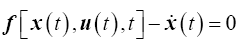   (10)

where the final time t_f is fixed, the final state, x(t_f), is free to vary and the state and control is not bounded. The terminal state weighting matrix, P, and the state weighting matrix Q are real, symmetric, positive semi-definite matrices and the control weighting matrix, R, is a real, symmetric, positive definite matrix.

The Hamiltonian for the tracking problem is defined as

   (11)

Where the Lagrangian is

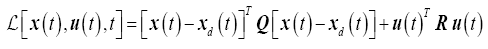   (12)

And the augmented state is

   (13)

The necessary conditions for optimality are

State Equations

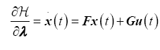   (14)

Co-State Equations

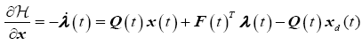   (15)

Optimality Condition

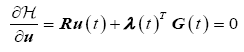   (16)

The optimal control law as a function of the co-state variable is therefore,

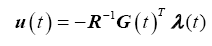   (17)

Substituting the optimal control law (17) into the state equations (15) and combining with the co-state equations (15), yields the Hamiltonian system

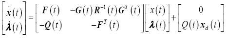   (18)

Note that this is a two-point boundary value problem in which we will need to integrate the co-state variables backwards in time. The terminal boundary conditions are

   (19)

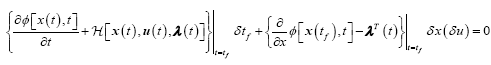
Because the final time is fixed and x(t_f) is free to vary, the following terminal constraint must then be satisfied

   (20)

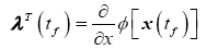
The partial derivative of the terminal cost with respect to the state is therefore

   (21)

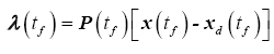
Assuming (21) holds for the entire interval, such that

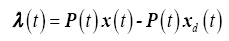   (22)

taking the time derivative

   (23)

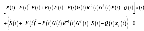
and substituting back into (18) yields the matrix differential Riccati equations (MDRE)

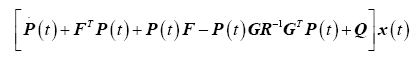
   (24)

Here we introduce the tracking variable and its derivative as

   (25)
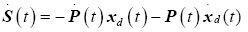   (26)

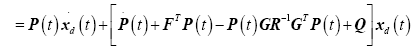
Substituting (25) and (26) into (24) results in

   (27)

The optimal state and desired trajectory cannot be zero for the entire interval; therefore (27) can be partitioned into two separate equations and integrated independently.

   (28)
   (29)

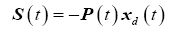
Rewriting the terminal condition for the tracking variable from (21) is simply

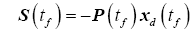   (30)

The optimal control law (17) is now written in terms of the Riccati variables and tracking variables, which can be further simplified into a feedback gain matrix, K(t), and a command signal, v(t),

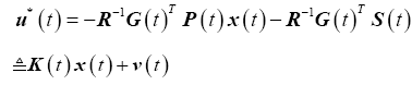   (31)

Delayed position state feedback

The linear quadratic tracking controller (LQTC) is shown in Figure 4. A delay of 150 ms is added to the position state feedback to appropriately model the neural transmission delay observed with smooth pursuit eye movements.

Figure 4: Optimal LQTC with Delayed Position Feedback.

The algorithmic steps involved are to numerically integrate the Riccati equations (28) and the tracking equations (29) backwards in time. These values can then be used to solve for the optimal state trajectory by substituting the optimal control (31) into (14) and numerically integrating.

   (32)

The optimal control (31) is now solved using the optimal state trajectory found in (32).

Application development

To help facilitate the selection of weighting values, a real-time application was built using Wolfram Mathematica to quickly test the response of the tracking algorithm for various waveforms with various frequencies as shown in Figure 5. The user may select the initial condition of the eye and the desired magnitude of the waveform. State, control and terminal-state weighting matrices can be inputted directly. The user may increase the position feedback delay gradually to effectively test the stability based on the chosen parameters. Four different plots are available as a visual aid to the designer. The State plot gives the response in terms of eye position and velocity. The phase option shows the phase portrait of the states and the Lyapunov stability of the system. The control selection shows a plot of the optimal control computed for the system. Finally, the MDRE option allows the designer to see both the time course of the numerically integrated Riccati and Tracking variables.

Figure 5: Linear Quadratic Tracking Application.

Closed loop unity feedback control effects of time delay

Figures 6 and 7 illustrate the destabilizing effect neural transmission delays have when introduced into the position feedback of the Wertheimer model. The values for the delays shown in Figures 6 and 7 are well below those observed with smooth pursuit eye movements.

Figure 6: Ramp response for closed loop unity feedback system A) with zero delay, B) with delay of 20 ms.

Figure 7: Oscillatory response for closed loop unity feedback system A) with zero delay, B) with delay of 15 ms.

The delay values for the ramp response shown in Figure 6 and the oscillatory response shown in Figure 7 are well below those observed with smooth pursuit eye movements

Closed loop linear quadratic tracking control-no time delay vs time delay of 150 ms in position feedback

Experimentation of weighting values for tracking ramp and oscillatory trajectories resulted in the following numerical values for the state-weighting, control-weighting and terminal-state weighting matrices.

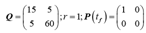   (33)

Overall, these weighting values provided the best all-around tracking performance for the continuous waveforms tested across frequencies up to 1 Hz.

Ramp Response (Figure 8)

Figure 8: LQTC ramp tracking with A) zero delay, B) 150 ms delay.

Target trajectory =20 t, Initial Eye Position=0°

Cosine Response (Figure 9)

A) Target trajectory = ;Eye starting position=3°

Figure 9: LQTC tracking of a Cosine with initial target error of 17° A) 0 delay B) 150ms delay.

B) Target trajectory = ;Eye starting position=20°

The optimal control calculated for when the eye initially starts on the target has an anticipatory effect. It senses the delay and adjusts its course accordingly as shown in Figure 11.

Figure 10: LQTC of Cosine with eye starting at initial target position A) 0 delay, B) 150ms Delay.

Figure 11: The predictive nature of the optimal control A) 0 ms delay B) 150 ms delay.

Sum of Sines (Figures 12 and 13)

Target Trajectory =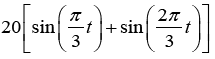 ;Eye initial position=0°

Figure 12: LQTC of the sum of Sines A) 0 delay, B) 150 ms delay.

Figure 13: Optimal control for sum of Sines A) 0 delay, B) 150 ms delay.

Product of Sines (Figures 14 and 15)

Target Trajectory= 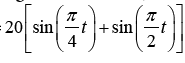;Eye initial position=0°

Figure 14: LQTC of Product of Sines A) 0 Delay B) 150 ms Delay.

Figure 15: LQTC Optimal control for product of Sines A) 0 Delay, B) 150 ms Delay.

Discussion

Weighting effects

The effectiveness of the LQTC is driven by the performance criteria specified in (9) which establishes tradeoffs between state and control. The state-weighting matrix, Q, specifies the relative importance between each state while the control-weighting matrix, R, establishes the permissible energy expenditure (a scalar value in this study). Consider the response of the LQTC with different stateweighting factors for an oscillatory input at different frequencies as shown in Figure 16. The relative tradeoff between position and velocity performance for different frequencies is a direct result of the weighting values and readily apparent by inspection.

Figure 16: Effect of state-weighting values on response with a 150ms delay.

Careful experimentation with different weighting values for multiple waveforms at different frequencies resulted in the values presented in (33). The effect of penalizing velocity more heavily than position, along with weighting the coupling between them, resulted in exceptional tracking performance.

Effects of initial eye position

The initial orientation of the eye in relation to where the target is presented affects the time in which the LQTC can fully pursue the trajectory. Figure 9 provides a good example of this issue. The difference between the position of the eye and the target trajectory is initially 17°. For the case with no delay, it takes five seconds for the tracker to fully engage the target and pursue it with minimal error. The addition of a time delay of 150 ms further exacerbates the situation requiring nine seconds for the LQTC to fully track the reference trajectory. Interestingly, if the initial eye position starts on the target as shown in Figure 10 for comparison, the tracker performs exceptionally, even for a delay of 150 ms this can also be observed for the ramp (Figure 8), the sum of sine waves (Figure 12) and the product of sine waves (Figure 14). This behavior is not surprising however. As mentioned earlier, smooth pursuit eye movements are commonly preceded by a saccade to rapidly position the eye to the target trajectory where it then switches control strategies to smoothly pursue it. The results presented in Figure 16, therefore, reinforce that fact.

Optimal control

Referring back to the optimal control law (31), the command signal v(t) depends on system parameters and future values of the reference trajectory, x_d(t). Having this knowledge as a priori, we can anticipate where we intend to go based on the current state of the system. This statement is directly supported by observing the optimal controls computed for the zero delay and 150 ms delay responses of Figures 11. In both cases, the LQTC effectively tracks the input. The major difference is the optimal control required to do it. The optimal control of Figure 11A is an exact replica of the desired trajectory. In contrast, the optimal control of Figure 11B leads the input to account for the neural transmission delay because it has prior knowledge of not only the trajectory to be tracked but also the current state of the system. In essence, the LQTC uses an internal representation of the system state and makes adjustments to improve behavioral performance. Figure 13, the optimal control for the sum of Sines and Figure 15, the optimal control for the product of Sines, further validates this point.

Model weakness

The LQTC requires that all states are measurable and available for feedback. Additionally, it requires prior knowledge of the desired trajectory which might not always be the case. Finally, the controller assumes that the inputs to the system and the measured states are noise free. Because sensorimotor systems are inherently noisy, it seems that the logical progression would be to introduce an estimator. This is left for future work.

A linear quadratic tracking control algorithm was developed to study smoothly pursuing eye movements in the presence of 150 ms neural transmission delays. The excellent tracking capabilities of the controller were presented for a variety of input reference trajectories with varying frequencies. The resulting optimal control was shown to have an anticipatory quality resulting from prior knowledge of the reference trajectory and an internal representation of the system state. Finally, the effects of initial eye position in relation to the start of the target trajectory were discussed. The results support the requirement for switching control strategies in which a saccade precedes the smooth pursuit.

This work is financially supported in part by QCI, Inc. of Seekonk, MA