Journal of Geology & Geophysics
Open Access

Integrating Geomechanics in Full-Field 3-D Reservoir Simulation in Bonga Field, Niger Delta

Author info »

Introduction

The goal of a reservoir study is to understand and describe the dynamic behavior of a hydrocarbon reservoir by properly integrating all the available geological, geophysical, petrophysical and engineering information so as to predict the future performance of the system under different development and production strategies. To that purpose, it is common practice to rely on a reservoir model that can handle and process a large amount of data. This model is generated to accurately reproduce the structural and petrophysical properties of the hydrocarbon-bearing formation and to describe the fluid dynamics taking place within the reservoir. Ideally, the same model should be further extended to account for the rock mechanical properties, to calculate stresses and deformations induced by operating the reservoir. In this way, all relevant aspects (static, dynamic and geomechanical) would be incorporated into one comprehensive model, by which not only single phenomena but also their mutual interactions, as they occur in the reservoir, could be investigated for forecast purposes and economic evaluations.

In recent years, the need for more accurate modelling, with a higher level of details so as to capture most of the reservoir geological and geomechanical features and to describe complex interactions among rocks, fluids and wells, are currently leading to the creation of software packages that incorporate all the subsurface disciplines and provide a common project environment for petroleum geoscientists and engineers. The coupling between fluid flow and geomechanics is required to model rock compaction effect on reservoir production performance. The remaining part of this section reviews the approximation method used in conventional reservoir simulator to model geomechanical effect, and a variety of proposed coupling methods.

In this study we address this limitation by using a commercial finite element pre-processor (Altair^® Hypermesh^®) and use the Coupled Geomechanical Reservoir Simulator, CGRS, a coupling module for geomechanical reservoir simulation developed at Missouri University of Science and Technology to convert several synthetic reservoir geometries from the finite element file format to the reservoir simulation grid file format [1,2]. We then study the effects of fractures on the drainage pattern of the reservoir. We use the commercial fluid flow simulation package Schlumberger^® Eclipse^® to investigate the effects of different amplitudes, wavelengths and height of generic anticline structures on the storability of CO2 in these reservoirs at different depths and under different injection rates. The results of this study may finally serve as a guideline for possible injection sites and scenarios resembling the cases presented here. The methodology presented in this paper further enables coupling between the reservoir simulation and the geomechanical analysis whereby both simulations use the same discretization minimizing the use of interpolation algorithms.

Field location

This study was carried out using Deepwater Bonga Field, located 120 kilometers offshore in the Gulf of Guinea (Figure 1), is the first major deepwater field operated by Shell in West Africa in partnership with ExxonMobil, Total and Agip, and under Production Sharing Contract with NAPIMS. Water depths at Bonga ranges from 945-1158 meters (3100-3800 ft).

Figure 1: Diagram showing the location of studied area and the Niger Delta mega-structural framework.

Research Methodology and Materials

Database

The study field is covered by 3D seismic data with an area of ~1814 km2 that was acquired in 2008, and reprocessed though pre-stack depth migration in 2012. We analyzed the pre-stack, depth-migrated 3D reflection seismic data set. The average dominant frequency of data was 30 Hz. The seismic data were used to detect subtle faults and large-scale fractures. Geophysical logs of AC, DEN, CN, and GR from 6 wells (BON--01, BON-3ST-1, BON-04, BON-4ST1 and BON-05) were collected and used in this study. The 6 m cores from two cored wells were observed and analysed. Geophysical logs and core observation data were used to identify the features, e.g., fracture density and fracture dip angle of small-scale fractures at the borehole scale.

General methodology

The methodology used in this case study integrated a wide range of measurements and associated studies. The first stage was to analyse well information, primarily wireline logs, outcrops, image logs and core data, plus all available dynamic data, such as production data from analogue fields and well tests from nearby wells, in order to analyse the role of natural fracture and fault network on fluid flow. The second stage was to interpret seismic data and calculate both conventional seismic attributes (e.g., coherency, curvature, dip) and more advanced attributes (e.g., seismic facies analysis, inversions, anisotropy and diffraction studies) in order to detect the presence of sub-seismic faults and predict the preferential direction of open fractures.

The third stage was to perform geomechanical modelling and associated detailed studies to predict strain and stress, fracturation characteristics and faults displacements. Once these studies and analyses have been completed, a conceptual model can be built that will provide the basis of a Discrete Fracture Network (DFN) model, which can be fine-tuned and up-scaled with well information to obtain reliable and coherent fluid simulation models. Summarizes the general fracture characterization workflow that has been performed in this study.

Geological framework for interpreting stress data

The state of stress that exists in a rock today is a function of its geological history, rock properties and the boundary conditions that are currently being applied. Knowing this, it is apparent that predicting a stress state in a rock today is not practically given the complex geological history that ancient’s rocks has endured. Consequently In situ stresses must be measured. However, to interpret these measurements a geological framework that considers geological history, rock properties and boundary conditions is required (Figure 2).

Figure 2: 3D view of the structural framework of the model. The mesh grill top and bottom (blue and yellow) are model boundaries whereas the different coloured vertical pillars are the faults interpreted along the entire 3D structural grid. Horizons are color-coded by depth. Faults are individually assigned a unique colour automatically.

Rock mechanical properties

The rock mechanical properties required for the finite element modelling, i.e., Density, Young’s modulus and Poisson ratio, are calculated from the 1-D geomechanical models using calibrated log based relationships.

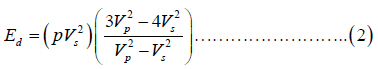
The continuous estimation of static log-based mechanical properties of the formation was done through the application of published empirical relationships (Equation 1 to 4) between static (laboratory measurements) and dynamic (derived from wireline logs) properties. Wireline log data from the five offset wells have been used to determine the Dynamic moduli using distinct empirical relations developed for each lithology shale mudstone and sand. Dynamic Young’s modulus and Poisson’s ratio were calculated using longitudinal slowness, transverse slowness, and bulk density data. Logging data were used to explain the continuous rock mechanics parameters of a single well’s profile. Young’s modulus and Poisson’s ratio were obtained as follows [3]:

Young′s modulus :

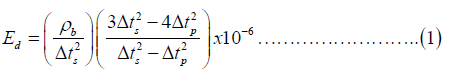
Therefore, when converted to velocity,

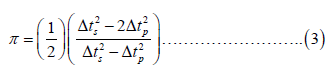
Poisson′s ratio :

Therefore, when converted to velocity,

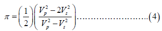
Where Δtp is compression slowness,μs/m; Δts is transverse slowness, μs/m; is density,g/cm³; Ed is Young’s modulus, MPa; μ is Poisson’s ratio. The variables ρ, V_p and V_s represent bulk density, compressional velocity and shear velocity respectively. E_d is Young’s modulus, MPa; μ is Poisson’s ratio.

The geomechanical properties required for the finite element simulations, i.e. Young’s modulus, Poisson’s ratio and material density were upscaled at each well location to a vertical resolution comparable to the FE mesh. Based on these considerations, the rock mechanical properties are averaged arithmetically to an upscaled log resolution varying between 150 m in the coarsely meshed over and under-burden and 20 m in the more finely discretized reservoir layers. After upscaling the rock mechanical properties, the rock densities, Young’s modulus and Poisson ratios are mapped onto a 3D grid. The 3D grid is a grid that comprises all the structural detail of the model, including all the relevant faults and horizons.

In some sections, where the density data is unreasonably low or high (due to poor quality density log from an enlarged hole) or is not available, the density log is interpolated by a best-fit line or by using pseudo density from the acoustic log using the Gardner’s relationship. By using all of these, the magnitudes of principal stresses were determined using the stress polygon method [4]. Then vertical and horizontal stresses, and stress directions, were estimated, especially around faults, using various techniques.

Pore pressure estimation

To complete the determination of stress state (Figure 3), knowledge about pore pressure is required. Direct measurements of formation pressure were available in the reservoir formations for most of the wells used in the present study. In the overburden sections, mud weights and drilling experience have been used to estimate the pore pressure. We inferred a hydrostatic pore pressure regime down to approximately 3000 m TVDSS, which is in line with the mud weight used to drill the shallow hole sections and the reported drilling events.

Figure 3: Plots of the principal stress magnitudes and the pore pressure as function of depth for BON-3ST1 well. The MW displayed used to drill this well (bright green) and the formation pressure measurements. Note: ( ) Hydristatic Pressure; ( ) Pore Pressure; ( ) Fracture Pressure; ( ) Overburden Pressure.

3-D geomechanical model construction and calibration

The accuracy of every 3-D geomechanical model lies in the availability and detailed generation of 1-D geomechanical models constructed from best quality available offset well data. Wells typically hold a multitude of partly high-resolution data sets including wire-line logs, well tests and in many cases rock strength measurements obtained from core plugs, which are then combined with the drilling experience for calibration, to build 1D geomechanical models. The input data for the three dimensional geomechanical model of the field is based on the individual 1-D geomechanical models from the following five offset wells: BON-01, BON-3ST-1, BON-04, BON-4ST1 and BON-05.

The geomechanical model is composed of the magnitudes and the orientation of the three principal stresses (S_Hmax, S_TTT and S_v), the pore pressure, and rock properties such as the Uniaxial Compressive Strength (UCS), Poisson’s ratio (μ) and Young’s Modulus (E). Based on data from wells across the field under study, the team proceeded to construct an initial Mechanical Earth Model (MEM), a quantitative representation of the stress state and rock mechanical properties of the interval of interest.

The available bottom-hole pressure data, mud weight, Modular Formation Dynamic Tester (MDT), and Formation Integrity Test (FIT) and MiniFrac data data recorded in wells were compiled. From these, overburden stress, pore pressure, Shmin and S_Hmax parameters were estimated and calibrated with MDT and FIT data.

Coupled 3D geomechanical modeling

Conventional reservoir simulators, designed to model changes in permeability, porosity, reservoir pore pressure and temperature under flow conditions, have no way of accurately modeling geomechanical stress and strain. While a typical reservoir simulator can apply a simple vertical stress to the model, it cannot handle the full stress tensor, which includes horizontal components, as well. As such, it cannot predict the failure behaviour of faults reliably, and cannot identify potential leakage pathways or compartments as pressure change over time. To achieve a full characterization of stress and strain throughout a complex geological structure, 3D geomechanical modelling is performed separately. However, to obtain meaningful production forecasts and properly value fields, the geomechanical simulator must be coupled with a traditional reservoir simulator.

The most effective approach is two-way coupling, which establishes a full iterative loop between simulators. With this approach, the team first modelled complex pressure changes across the field, caused by water injection, natural variations in porosity and permeability, and depletion due to production using the ECLIPSE industry-reference reservoir simulator.

Model calibration

The fundamental purpose of calibrating the static geomechanical reservoir model is to correlate the model to reality. The setup of a geomechanical model always requires some assumptions to be made, for instance regarding poorly constrained parameters. These assumptions are mandatory to setup the model, but inherently bear uncertainty. In order to counteract and reduce this uncertainty, the modeling results are compared to local measurements in a process referred to as calibration or validation of the model.

Appropriate data for the calibration process includes all types of stress and fracture measurements (data) in the reservoir. Stress data for calibration purposes was derived by In situ measurements. One of the most frequently available stress information is the magnitude of the least principal stress measured from SCAL data. Within the calibration process all stress magnitudes and orientations measured in the field, as well as fracture characteristics are compared to the respective modelling results.

Reservoir simulation

The ultimate objective of this workflow is to derive dynamic models that are able to reproduce past individual well performances without the need for any time-consuming history matching. This provides an additional validation of the fracture models derived using the CFM approach. Using the reservoir parameter models generated in steps 2 and 3, both black oil and compositional reservoir simulations were run to verify that these models would produce a history match to the production data.

Black oil reservoir simulation of the ‘Bon’ field production: In a black oil simulator, where the two main fluid phases are oil and water, the complex effects related to the injection of CO₂ are not considered. In the case of the ‘Bon’ reservoir, CO₂ injection did not yet occur and therefore the reservoir model could be validated with a black oil model. The aspects related to CO₂ injection will be considered in the next section using a compositional simulator.

The three major reservoir properties needed for reservoir simulation are permeability, porosity, and oil saturation. Given the presence of the fractures with high connectivity, the matrix permeability is expected to be enhanced. The degree of this permeability enhancement depends on the fracture density. Given the extensive fracturing present in the ‘Bon’ formation, there is no evidence of a dual porosity or dual permeability medium, and the reservoir appears to behave as a single porosity medium with an enhanced effective permeability. The matrix porosity seems to provide the storage for the oil, which has a tilted oil-water contact. Water production rates indicate that the ‘Bon’ formation has a strong aquifer, resulting in a pressure drop of less than 100 psi throughout the Formation. Consequently, water drive is considered the primary producing mechanism in the reservoir. Initial water saturations (Swi) are between 12.5% to 22.1%, and residual oil saturations (Sro) are between 28.7% and 56.3%. Measurements and tests of the ‘Bon’ Formation show that the initial reservoir pressure at a depth of 5400 ft is approximately 2350 psi at a temperature of 190ºF. Analysis of producing wells in the ‘Bon’ Formation shows that all of the production occurs in section 10, near the crest of the structure. Oil producing wells exhibit a fairly good production history for the first 2 years, followed by a rapid breakthrough of water. The oil production is replaced by a high water production, which confirms a very high mobility of water in the reservoir.

The dynamic model uses the derived matrix porosity and oil saturation as input in the reservoir simulator. The key reservoir property is the effective permeability, as the dynamic model uses a single porosity system. In this case, the reservoir permeability is simply the effective permeability computed as follows:

K_eff=K m+ C • f

Where

K_eff: Effective permeability of the combined matrix and fracture flow in millidarcies

K_m: Matrix permeability in millidarcies

f: Fracture density [number of fractures/meter]

C: Scaling factor to be estimated by history matching

The matrix permeability and fracture density were estimated in the previous steps, and the scaling factor is estimated during the history matching process.

The history matching process consists of finding three reservoir parameters that are unknown: 1) the scaling factor C required computing the effective permeability, 2) the relative permeability curves, and 3) the strength of the aquifer. After a few tests, these three unknowns were easily estimated and the individual well performances of all the wells were matched. The dynamic model allowed a better understanding of the current fluids distribution. This dynamic model validated the geologic and fracture models, and we can use it for various reservoir management strategies, including CO₂ injection.

Results, Discussion and Achievements

Reservoir property models

A geologic model was developed from previous petro-physical evaluations of the five wells. Figure 4 provides 3-D view of (a) Fault plane map (b) Structural Model (c and d) lithofacies, at the reservoir levels (Miocene to Pliocene). Layering is evident as is lateral variation and heterogeneity (Figures 4-6).

Figure 4: 3-D view of (a) Fault plane map (b) Structural Model (c and d) lithofacies, at the reservoir levels.

Figure 5: Spatial distribution of (a)Total porosity, (b)permeability, (c) Poisson ratio and (d)Young Modulus on fault faces [MPa].

Figure 6: Spatial distribution of (a) Total porosity and (b) Permeability on fault faces.

Geomechanical analysis and properties

In situ stresses profile: The calculated magnitudes of the three principle stresses in the Bonga Field resulted that, S_hmax was found to be the higher principle stress, and the magnitude of the vertical stress was found to be greater than the minimum horizontal stress, indicating that a normal stress regime (S_v>S_hmax>S_hmin) dominates the field (Figure 7).

Figure 7: Pressure Profile and Stress profiles of BON-3ST1 well indicating a normal stress regime (Sv>Shmax>Shmin). The blue circles represent the Formation Fluid Pressures (RFT), and triangles indicate FIT pressure (the stresses are calculated using the elastic moduli estimated by the empirical equations. Note: ( )Sv; ()SHmax; ( )Shmin; ( )Pp.

The calibrated stress profiles for the BON-3ST1 well was prepared for interpolation into the geomechanical model, and the stress initialization distribution in the geomechanical model is shown in Figure 7. The boundary conditions for the global model were set as fully constrained bottom and lateral surfaces.

In situ stress magnitude

The distribution trend of Shmin magnitude was similar to that of S_Hmax, that is, lower in the central part and fault zone and higher in the surrounding area. The magnitudes were mainly between 36-65 MPa and the average stress gradient was 1.47 MPa/100 m. For vertical principal stress, the magnitudes were about 70-90 MPa, and the average stress gradient was 2.25 MPa/100 m. Overall, horizontal differential stress did not exceed 30 MPa and was generally below 20 MPa. Again, the distribution trend was one of being lower in the west and higher in the east. Within the target layer, if the vertical principal stress is greater than the horizontal stresses, this belongs to the normal-type of In situ stress.

The distribution of In situ stress orientations

The overall orientation of S_Hmax in the study area was NEE-SWW to SEE-NWW with a measured range between 58°-238° and 103°-283°. In the central region of the study area, the orientation of S_Hmax was closer to E-W, between 75°-255° and 96°-276°. In the western region, the orientation of S_Hmax was closer to NE-SW, between 58°-238° and 88°-268°. In contrast, orientations in the eastern region gradually rotated toward the SE-NW (99°-279°). The orientations of Shmin and SHmax were perpendicular, and the overall Shmin orientations were from NNW-SSE to NNE-SSW.

Within a fault block, the orientation of S_Hmax was relatively uniform and the variations were even. In contrast, changes in orientation were most obvious between different fault blocks. The non-uniform stress orientations were caused mainly by lithofacies heterogeneity and fault distribution. The former caused small, but consistent changes in the stress orientation within a fault block; the latter caused obvious deflections of the stress orientation. Consequently, there were large differences in stress orientation between fault blocks on either side of a fault.

Analysis of inter-strata In situ stress

Inter-strata In situ stress affects the height and direction in which fractures extend and expand, which is important to reservoir modelling. The combined Petrel and ANSYS modelling techniques made it possible for the predicted stress field obtained by numerical simulation to be used as a type of geological information for inputting into the 3D geological model. In turn, the characteristics of the stress field profile could be presented in detail in the Petrel grid (Figures 8 and 9).

Figure 8: 3-D view of PP, Sv, Shmax and Shmin models of Miocene to Pliocene Agbada Formation reservoirs (Each geobody represents its spatial distribution within the formation along the X-Y-Z axis of the modeled grid). The measured and modeled magnitudes of both horizontal stresses were compared and show that the respective deviations are always less than 4MPa. It also indicates the improvement due to calibration by additionally plotting the results of the default model (Figure 9).

Figure 9: Spatial distribution of PP, Sv, Shmax and Shmin on fault faces [MPa].

In the field profile, the In situ stress magnitudes of the Structure varied greatly with significant differences in inter-strata In situ stress. This was because a quantitative relationship exists between the rock mechanics parameters (especially Young’s elastic modulus) and the In situ stress magnitudes. Such inter-strata variations in In situ stress directly relate to the heterogeneity of the reservoir’s rock mechanics parameters [5].

Horizontal differential stress is the key actor controlling volumetric fracturing. A complex network of seams is easily formed when the differential stress is small; otherwise, a unidirectional fracture that is parallel to the S_Hmax will form instead. On the other hand, potential extensions of fracture height and length are mainly controlled by the distribution of the minimum principal stress above the fractured sections of the layer and the S_Hmax orientation respectively.

As the dominant fault and fracture networks trend E-W and NE-SW, it is most likely that the pre-existing set of fractures will open depending on their susceptibility.

Static elastic properties

The spatial distribution of the static Young’s modulus (E_d) and Poisson’s ratio (μ) values were obtained after the seismic interpretation and integration of the area’s seismic attributes. The elastic modulus varied mainly between 37-62 MPa, and Poisson’s ratio was concentrated between 0.2-0.27. In the 3D space, the rock density was between 2.05 and 2.60 g/cm3. Differences in the elastic properties within and between fault blocks were clear. The elastic properties of the fault zone have a great influence on the results of stress modelling, but the current accurate acquisition of parameters is still a problem. Generally, the size of the grid in modelling software is larger than 20 m, but the width of most faults in study area is smaller than this value. Therefore, it is difficult to accurately reflect the change of mechanical parameters of fault zones by seismic attribute technique. According to previous studies [6], the fault zone can be defined as a weak/soft zone, and its elastic properties are different from those of the surrounding rocks. In this study, the Young’s modulus of fault zones is 50%-70% of the surrounding rocks. Moreover, the Poisson’s ratios in fault zones were larger than those of the corresponding rock stratum, and their differences were typically between 0.02 and 0.10. The Young’s modulus in the reservoir is significantly lower (^~10 GPa) compared with the overlying non reservoir units (40-90 GPa). From above, the 3D geomechanical parameters obtained from the seismic attributes were finally adjusted and corrected to obtain heterogeneous mechanical parameters of fault zones (Figures 10 and 11).

Figure 10: Spatial distribution of static Poisson’s ratio (μ)and Young’s modulus (Ed) in the entire model block calculated from seismic data and well logs and converted into static values using a genetic algorithm -ANN.

Figure 11: Spatial distribution of static Poisson’s ratio (μ) and Young’s modulus (Ed) on fault surfaces calculated from seismic data and well logs and converted into static values using a genetic algorithm -ANN.

Reservoir property model validation

Figure 12 shows the petrophysical logs resulted from the neural network modelling compared with the calculated logs and compared to the upscaled logs for both the predicted and the calculated properties. Each log track illustrates predicted log, calculated log, upscaled predicted log, and upscaled calculated log of porosity and permeability.

Figure 12: Logs showing the results of reservoir property model validation. Data illustrate predicted log, calculated log, upscaled predicted log, and upscaled calculated log.

Reservoir simulation

The ultimate objective of this workflow is to derive dynamic models that are able to reproduce past individual well performances without the need for any time-consuming history matching. This provides an additional validation of the fracture models derived using the CFM approach. Using the reservoir parameter models generated in steps 2 and 3, both black oil and compositional reservoir simulations were run to verify that these models would produce a history match to the production data (Figures 13).

Figure 13: Influence of coupling on the pore pressure distribution.

Validation of the reservoir model

The validation of the reservoir model is shown in the figure below (Figure 14).

Figure 14: Bottom hole pressures as a function of time showing comparism between actual, simulated pressure measurements using Two-way, coupled geomechanical modelling and traditional reservoir simulation. Note: ( ) Historic BHP; ( ) Reservoit simulation; ( ) Two-way coupling.

Conclusion

The aim of the study is to demonstrate the need for an integrated approach in the construction of hydrocarbon reservoir models. In fact, a truly integrated workflow leads to an overall improvement of the reservoir model from the static, dynamic and geomechanical point of view. The updates, revisions and modifications proposed at each step, including progressive adjustment of the model parameters in the calibration phase, are shared among the different specialists and coherency is inherently ensured.

During dynamic modelling, the engineers can provide the geologists with valuable information about the hydraulic connectivity among the geological bodies or through faults intersecting the reservoir. They can also offer feedback on the petrophysical parameters and their distributions based on the calibration of the global energy balance of the field, as the global pressure level is adjusted by modifying the pore volumes occupied by the different fluids.

The coupling between rock mechanics and fluid flow properties can have a significant impact on fluid dynamic simulations. For this reason, the calibration of a model, so that it can simultaneously reproduce the stress/deformation evolution and the production history, is deemed necessary. However, some geomechanical properties are directly connected with the static model parameters, so it is often possible that the calibration procedure involves modifications to the parameters of the static model as well. For this reason too, an integrated methodology is the only one guaranteeing a rigorous technical approach to reservoir studies.

The main advantage of a working philosophy that looks at the whole picture rather than at specific issues of a reservoir study is the possibility to set up a model which can be equally employed for the development and production forecast scenarios and for geomechanical purposes, such as subsidence predictions. Therefore, even if the need for a model capable to handle all geological, dynamic and geomechanical aspects is not envisioned when a new field study is undertaken, it is recommended that an effort is made to keep that option viable for the future.

Additionally, the cost of an incorrect production strategy due to an incorrect understanding of the geological features and settings, or due to failing to capture the main production mechanisms governing the field behaviour, is much more expensive than that of an integrated study.

The need for integration in reservoir modelling has been well perceived by scientists, who developed the theory and practices for making it a reality, but also by the various companies specialized in s o f t w a r e used for numerical simulation of various kinds. In fact, in the last several years, a continuous reduction of separate stand-alone software packages was observed. At the same time, a migration to single multifunctional software platforms was witnessed in the petroleum field, so that geoscientists and the engineers cannot only update data and share results with all users in a common working environment, but they can also use the same software and work in real time on the same project.

So the path for the creation of high-quality, reliable and versatile hydrocarbon reservoir models has been set and paved; now individuals and personal attitude to team working will make the difference. Computer tool to displays the stress tensor in terms of its associated dilation and slip-tendency distribution and the relative likelihood and direction of slip on surfaces of all orientations. The technique provides easy visualization and rapid evaluation of stress in terms of its potential for causing slip on individual faults or fault populations for use in seismic-risk and fault rupture-risk assessment.

References

1. Orlic B, Wassing BBT. A study of stress change and fault slip in producing gas reservoirs overlain by elastic and viscoelastic caprocks, Springer. 2013: 421-435.
2. Sathyamoorthy S, Olatunbosun O, Sabatini D, Orekyeh U, Olaniya E. Society of Petroleum Engineers, Nigeria Annual International Conference and Exhibition, Abuja, Nigeria. (2009).
3. Liu Y, Dong N, Fehler M, Fang X, Liu X. Estimating the fracture density of small-scale vertical fractures when large-scale vertical fractures are present. J Geophys Eng. 2015;12: 311-320.
4. Zoback MD. Reservoir Geomechanics, Cambridge University Press, Cambridge. 2010: 266-297.
5. Dee SJ, Yielding G, Freeman B, Healy D, Kusznir NJ, Grant N, et al. Elastic dislocation modelling for prediction of small-scale fault and fracture network characteristics. J Geol Soc London. 2007: 139-155.
6. Liu E, Martinez A. Seismic Fracture Characterization: Concepts and Practical Applications, Education Tour Series. EAGE Pb. 2012: 279.