Journal of Tumor Research
Open Access

Identification of Brain Tumor Detection from MRI Image Using Convolution Neural Network

Author info »

Introduction

One of the most complex systems in the body is the brain, as it functions with such a vast number of issues. Brain tumors grow because cells divide uncontrollably, resulting in an irregular pattern. The behavior of brain activity will be affected by the group of cells, and the healthy cell will be damaged. The manual segmentation and an assessment of intrinsic MRI images of brain tumors, on the other side, are a complex and time-consuming process that can presently only be conducted by specialist neurosurgeons. Digital image processing is a critical task in MRI image processing. X-ray images are commonly used in therapeutic medicine to evaluate and recognize tumor growth in the body. A brain tumor affects both children and adults [1]. Tumors result in high levels of cerebral fluid spread throughout the skull stem. Inside the skull, cancer grows, interfering with normal brain function. A tumor could be the cause of cancer, a leading cause of death that accounts for approximately 15% of all global deaths [2]. The National Cancer Institute (NCI) will detect 22,070 new variants of brain cancer and other central and peripheral nervous system disorders in the United States in 2009. The American Brain Tumor Association (ABTA) states that 63,930 fresh cases of an initial stage of brain tumor were reported by the American Brain Tumor Association [3]. Figure 1 demonstrates a Brain Tumor’s Presence. At the moment, there is no easy way to determine the root origin of brain tumors. However, the result of radiation contamination during MRIs, X-rays, and computerized tomography scans. Severe seizures, and loss of brain function, are, however, the result of radiation contamination during MRIs [4], CT scans, and X-rays. Brain severe seizures characterize tumors, loss of brain function, consciousness, neurological disorders, numbness, speech problems, hormone abnormalities, and personality changes are all indications of brain tumors. The most recent traditional diagnostic method relies on human experience from the perspective of choice in the MRI scan, which raises the chances of false detection and cerebrum tumor awareness. That used, Digital Image Processing (DIP) allowed for easy and reliable spotting of tumors [5]. Medical image segmentation was a crucial part of the study because it raised several challenges related to accurately segmenting images in brain illnesses. Radiologists use a CT scan and an MRI to examine the patient visually. MRI images are being used to investigate the cerebrum structures, size of the tumor, and location [6]. Imaging is essential in the diagnosis of brain tumors. They frequently find tendon MRI is either iso or hypo tense. There are instant transitions through grey tones when the features are referred to as sides. The grey tone fluctuations in the photos help edge recognition techniques convert images to Edge features. The optimization map is formed beyond altering the physical properties of the main image. The radiologists’ MRI pictures revealed facts such as tumor location, a straightforward technique to diagnose the tumor, and how to prepare for the surgical surgery [7]. Figure 1 shows the vitiate section of the cerebrum is detected from the tumors in the brain region.

Figure 1: (a) Normal Brain, b) Benign Tumor, c) Malignant Tumor.

In MRI, three-dimensional reconstructions of the hidden organ are utilized to create a strong magnetic field and radio waves. Ionizing radiation is not a problem with MRI technology [8]. The absence of ionizing radiation is a significant advantage of MRI scanning. Computer vision algorithms improve the diagnosis process of MRI scans. The cerebrum images play a crucial job in cure image processing [9]. Cure identification is made feasible by revealing the interior mechanics of the human being’s hidden structure through the generation of cure images. Both patients and doctors benefit from the processing of medical pictures. That is one of the most common optical computer vision applications that utilize various processes to improve the precision of an image. For decades, image processing has been used to identify brain cancers. Many of the semiautomatic strategies for identifying cerebrum tumors, as well as several impulsive computer vision techniques, have been identified by researchers. However, because the presence of roar and poor dissimilar pictures are familiar in medical images, the majority of them do not include efficient and accurate results [10]. Brain tumor segmentation is complex due to the complicated brain structure, and detecting tumors early and reliably is difficult. The diagnostic gadget is crucial for malignancies, edema, and necrotic tissues. Cancer is sensitive to harm a standard cerebrum stem, resulting in swelling, pressure on areas of the cerebrum, and increased force put on the skull. Presently, mathematical models motivated personalize streams, and a wide range of arithmetical trends are used for the storage of patient data [11].

Challenges

The difficulties in detecting brain tumors stem primarily from the tumors’ wide abnormality in form, constancy, dimension, position, and diverse aspect. For medical practitioners and pathologists, detecting a brain tumor from a patient’s different symptoms has always been a crucial concern for diagnosis and treatment planning.

Problem statement

The majority of tumors nowadays are life-threatening, with brain tumors being among them. As we all know, brain tumors can come in any shape, size, location, or intensity, making detection and diagnosis extremely challenging. Manual tumor identification from MRI pictures is spontaneous and different from specialists depending on expertise. The other factor is the failure of separate and precise quantitative metrics to identify the MRI images as a brain tumor or not. Many patients die as a result of late detection of tumors, particularly brain tumors. Early detection and classification of brain tumors improve the chances of treating and curing patients. As a result, automated brain tumor detection using CNN helps to alleviate key concerns and deliver superior outcomes.

Research objectives

Given the preceding facts and descriptions, the thesis work’s research objectives are as follows: To collect images and form an annotated tumor dataset containing various MRI images. To develop a more effective and accurate Convolutional Neural Network Model for identifying and detecting brain tumors. To evaluate a proposed model based on validation accuracy and minimum loss with the state-of-art model. The following is the structure of this paper: First, a basic overview of brain tumors. Section II contains related work. Section III is Research Methodology; Section IV contains Dataset and Evaluation Metrices, Section V includes Result and Performance Analysis, Section VI consists of a Conclusion, and Section VII Future scope. Our approach, which outlines previous studies using the same information, can segment and anticipate the bad shape of the three brain tumors.

Related work

Before the widespread adoption of deep learning systems, computer vision researchers devised several innovative and slightly successful methods for brain tumor detection. Initial classification methodologies necessitate domain experts to identify meaningful features for the desired classification objective. Such plans are created to extract these features from the image, and then evaluate individual differences using statistical analysis or a deep learning technique (Arya Sharma).

Islam, et al. recent use of MRI in informatic computer vision [12]. Magnetic Resonance Imaging (MRI) allows for the rapid determination and localization of cerebrum tumors. We intend to categorize cerebrum scans into eight classes, with seven specific, numerous groups of tumors and one indicating a healthy cerebrum. The univariate procedure was used for the proposed classification strategy has been validated.

Joshi, et al. the segmentation of brain tumors has received much attention in medical imaging studies in recent years [12]. Only quantitative disease modeling measurement allows for monitoring and recovery. MR is usual in the beginning phases. The condition is more vulnerable to identifying brain problems such as cerebral infarction, brain tumors, or infection.

Deepak, et al. backpropagation of the neutrals order process is used to describe a path for the order of MRI pictures [5]. Image enhancement, registration, nature identification, and isolation techniques are used to create the strategy.

Morphological procedures and threshold values are taken into account during the segmentation process. The Neural Network (NN) technique of the backpropagation is used to assess these training images and experiments to recognize the existence of a cerebrum tumor.

Sasikala, et al. discover a new strategy for autonomous tumor detection employing a deep neural network for glioblastoma detection [10]. It uses a final layer that implements quick segmentation, which takes near about from 24 seconds to 3 minutes for the full lungs region.

Kiranmayee, et al. proposed a method for detecting brain tumors that included both training and testing [11]. The proposed algorithm’s functionality has been confirmed by developing a blueprint application. The prototype results suggest that in the sphere of pharmaceutical services, the option of emotionally supporting networks can be coupled to improve service quality.

Arya, et al. [12] proposed a histogram-based, watershed, SVM-based segmentation, and MRF segmentation can be a module to achieve greater accuracy and a lower rate of error.

Demirhan, et al. approach partitioning algorithms for MRI categorization of cerebrum tumors CSF, edema, WM, and GM are studied using SWT, LVQ, and grey matter [3]. The grey matter had an average similarity of 0.87 percent, CSF had an average similarity of 0.96 percent, edema had an average similarity of 0.77 percent, and the white matter had an average similarity of 0.91 percent.

Aneja, et al. approaches the FCM and partitioning algorithm, which works with the FCM cluster to counteract image roar [1]. The cosine similarity parameters, latency, and 0.537 percent converging regression coefficient generate the segmentation value.

Kunam, et al. Apriori k-means grouping, k-nearest neighbor classification, fp tree-based association gathering, and random forest are statistical approaches used to analyze such procedures using inside and outside assessment techniques [6]. The following strategies are used in conjunction with the experiment described in this paper: There are three distinct approaches, each with its own set of data mining algorithms.

In almost every situation, the interface has an overhead of less than 10%.

Each of the four statistical approach techniques achieves an excellent equivalent act.

If a decision tree construction algorithm occurs, spectacular execution will necessitate a combination of varied strategic swings.

Siar, et al. a tumor was detected using a Deep Convolutional Neural Network (DCNN) [10]. The DCNN was the first location where who discovered images. The classification of the Softmax Fully Connected (SFC) plate, which was used to classify the photos, accuracy was 98.67 percent. The precision of the Convolution Neural Network (CNN) is 97.34% accuracy when using the RBF grasses and 94.24 % when using the DT analysis.

Methodology

ImageNet competition, Krizhevsky, et al. created a winning convolutional neural network that outperformed the previous stateof- the-art model [14]. Following this competition, the computer vision community recognized neural networks as state of the art, appreciating the power of convolutional neural networks in picture categorization.

Pashaei, et al. proposed to identify tumors from Image data, Ensemble Learning Machines (ELM) to categorize the visuals to their similar features extracted, and CNN to classify tumors, and they achieved a finding of 93.68 percent success rate using KECNN [15].

Seetha, et al. Contrast enhancement techniques to identify brain cancer and suggested an automated tumor detection method relying on the CNN model. Those who generated a vital precision of approximately 97% results refer to and use a CNN layer [16].

Ismael, et al. They developed a model for identifying brain cancer using morphological features and neural net methods [17]. They applied the area of study region of interest to split the cancers and based a neural net on identifying them, with an absolute precision of 91.9 percent. Gopal et al. suggested segregating brain MRI data employed cluster analysis and probabilistic reasoning with classification methods [18]. This work utilized an optimization algorithm and the evolutionary programming method. The initial phase of the process includes cleaning and vision improvement of MRI data.

The use of the discrete Fourier transforms to identify tumors was revealed by Sridhar, et al. [19]. The authors further demonstrated neural network-based tumor identification and matched the outcomes.

Dropout was introduced by Srivastava, et al. as a simple approach to prevent neuronal co-adaptation [20]. Dropout causes neuron units to become more independent rather than reliant on other neurons to recognize features by randomly dropping neuron connections with a specific probability. Maxout layers are similar to dropout layers in that they were created to work together. Several other authors have emphasized and explored the identification of tumors using various techniques and innovative technology.

Identification is amongst the most effective methods for identifying visuals used in radiography. Primarily classifying methods rely on a visual forecast for one or even more aspects, some of which relate to several groups. We discuss using CNN and VGG16 models with diverse data parameters to simplify neural net classification performance. Our suggested flowchart intends to recognize and classify brain cancer inpatient data, use the proposed approach of deep learning-based, and apply the CNN algorithm. Also, it contains different stages based on how this effort is built. Figure 2 shows the proposed flowchart for identifying brain cancer and its phases.

Figure 2: The flowchart of the brain tumor detection model.

Input

The MRI images are first acquired, and then they are fed into the preprocessing stage. It’s also confirmed that the person is fully fit and capable of undergoing an MRI scan with the doctor’s assistance and support. The current study uses a patient’s brain MRI images as input.

Image pre-processing

Image preprocessing is needed to optimize the image data, which improves certain image features that become critical for subsequent processing. The dataset can also be translated from its raw state for simple analysis. The dimensions of a tensor depicting a 64 × 64 image with three channels will be (64, 64, 3). Currently, the data is saved as JPEG files on a hard drive. All of the colors we come across are in RGB. Making the photos the same size is also a preliminary step in data preprocessing. The methods used for preprocessing are-

Importing libraries: TensorFlow, NumPy, Pandas, Image grid, Global, Matplot-lib, OpenCv2, and Sci-kit etc libraries imported.

Image resizing: Resize images to a pixel value in 0–1 of the shapes (240, 240, 3). Several data augmentation strategies, such as cropping, padding, and horizontal flipping, are applied to expand the testing data collection and provide broad input space for CNN and VGG 16 to prevent excessive fitness during the training process.

Importing augmented data: Augmentation data en¬hances original data’s value by incorporating information from primary and secondary data sources. Data is one of an organization’s most valuable resources, rendering data processing critical. The essential idea of data augmentation is this. We might have a dataset of photographs captured under specified data in the natural environment. The objective of channel estimation seems to be to alter the visuals so that Deep Convolutional or DL framework keeps failing to exist account for them. Some modified visuals can also be used as a training phase to mitigate such Deep Convolutional or DL model deficiencies. The ability to add image patches, pooling layers, key aspects, and geospatial data to pictures. This feature made it incredibly simple to use the program on a database of photos for data processing and feature detection problems. The Image Data Generator component in Keras’ deep architecture enables image data enrichment. We adjust for these circumstances by using synthetically changed data to train our neural network as shown in Figure 3.

Figure 3: Real image of brain.

Convert binary images to gray scale images: Each pixel in a source image has only two values 0 and 1, which correlate to black and white. There are 256 different grey colors in a greyscale image since each pixel has a particular number of sources of evidence, likely 8 per pixel. Orignal impressions convert to grayscale images using Scale 0.7 shown in Figure 4.

Figure 4: Grayscale image of brain.

Thresholding: In thresholding, every photon image is determined to the target value. Whenever the euclidean distance is much less than a threshold, the maximum value is set to 0. Otherwise, the ultimate value is set to 0. Selecting a threshold value T and then putting every intensity value far below T to 0 but all pixels higher than T to 255 is a similar instance. We will produce basic features of the data in this way shiwn in Figure 5.

Figure 5: Images showing thresholding and inverse thresholding.

Morphological transformation using erosion and dilation: Morphological transformations are transparent operations that have been dependent on the shape of an image. They usually take place on binary images. Those that require two inputs, one is the image, and the second is called a structuring factor or kernel that determines the operation’s existence [21]. Erosion erodes foreground object borders. Each pixel value of 1 or 0 in the original image can only be regarded as 1. If all pixels under the kernel have been eroded, it is not 1. Therefore, who would remove the pixels along the border based on the kernel size. The thickness or height of the first object either decreases or only decreases in the white area in the image, as shown in Figure 6. We have thus used the brief white sounds to remove them.

Figure 6: Image after removing erosion and dilation.

Canny edge detector: The detector is a multi-stage contrast enhancement generator that identifies a diverse range of lines in frames. A Detector is a sub heuristic that senses the boundary of every input data. It includes the various efforts being made to detect a physical object. Because image quality impacts feature recognition, the first step is to remove the noise with a 5x5 Gaussian filter. To locate the tumor’s shape after an image is applied to the detector. The canny auto function is used to dynamically measure the lower and upper threshold values. Image noise is minimized using the Gaussian function. Possible boundaries are being narrowed to 1-pixel lines, permanently removing objects of an average filter [22]. Finally, applying hysteresis thresholding on the gradient magnitude, edge pixels are maintained or eliminated shown in Figure 7.

Figure 7: Auto canny of brain.

Tumor contour: Contours are defined as the kind of lines connecting all locations to the same resilience along the object’s border. Contours can assess patterns, identify the diameter of importance, and recognize obstacles. The active contour model is used to segment the entire tumor section to solve these issues. Forming a circular area around the tumor region detects the original Contour for Active Contour model. The radius of the circular area contracts or expands depending on the tumor’s form. Figure 8 illustrates the object detection of contour images as shown in Figure 9.

Figure 8: Final image of contoured image.

Figure 9: Images label with tumor yes and no.

Resize the images: We divided the group into different frames: training and testing. Researchers will be using Keras TB of data to generate the tags into discrete clusters and NumPy resonators. Because so many of the images were of different sizes. Before preprocessing, All amplified pictures are indeed enlarged to 240 × 240 pixels for CNN as well, as 224 × 224 pixels for VGG-16.

Splitting dataset: Dataset decomposed into three data sets training data, testing data, and Validation Data. We used 70 percent of the available data for training data, 15 percent for test sets, and 15 percent for the validation set.

Convolution neural network

A separate series of filters, usually hundreds or thousands, are applied by each layer on a CNN and merge the effects and feed the output to the next layer of neural. Throughout the preparation, a CNN automatically finds the core beliefs for these filtrations [23]. A kernel can be thought of as a tiny matrix sliding over a big image between the left, right, and center. Each print is a factor that is the main point of the kernel, and the output is processed at every individual frame as in source images. Example-convolving an image 3 × 3 region with a 3 × 3 kernel (mathematically referred to as operator) [2].

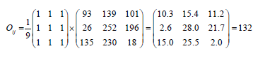
The bitmap image at dimensions (i,j) of the output visual O is fixed to Oij=132 after implementing this convolution. CNN will gain knowledge of filtration to reduce the dimensionality and kernel frameworks in the narrower network layer. After that, use sides but also constructs as essential elements to detect high-level artifacts in the network’s surface depth using convolutional filters, nonlinear mapping functions, pooling, and back propagations. There are several possibly the best convolutional neural network models, such as Alex Net, Google Net, and LeNet, which can be used to create this architecture. As seen in Figure 10, the architecture is being developed. To fit the developed model, despite adjusting several variables and verifying them, who recommended network design for the optimal outcomes. As illustrated in Figure 10, the Cnn model’s architecture consists of different layers, which each executes a distinct function and has another system.

Input layer: All images have been resized to 240 × 240 pixels, with a height of 240 pixels and a width of 240 pixels, and a depth of 3 (amount of feature networks).

Figure 10: Proposed deep CNN architecture.

Zero padding: We must pad the image boundaries to keep the initial image size when adding a convolution. The same can be said for CNN filters. We should pad our input along the edges with zero such that the output volume size equals the input volume size. We used pool size to perform zero padding on our photographs (2,2). Example-Consider the following graphic, which is expressed as a matrix [2] as shown in Figure 11. The picture is padded with zeroes, indicating the pool size (2,2) as shown in Figure 12.

Figure 11: 5 × 5 images in its matrix.

Figure 12: Images applied to zero padding.

Convolution: The convolution layer is the fundamental component of a CNN. Several K (kernels) learnable filters comprise the convolution layer parameter. Consider CNN’s forward pass [23]. We used 32,64 and 128 filters of different sizes in the convolution layer of our presented work (7,7). The receptive field [local area of input volume to which each neuron is connected] is the size (7,7). We used a (7 × 7) receptive field, which means that the image would bind each neuron to a 7 × 7 local area, resulting in 7 × 7 × 3=147 weights. We now have 32; 2-dimensional activation maps after adding all 32 filters to the input volume. Each entry in the output volume is thus the product of a neuron that only examines a small portion of the signal. The network “learns” filters that function when it sees a specific type of function in this way. As a result of the convolution process, the image size has increased to (238, 238,32), and the depth has increased significantly result of the filter used.

Stride: Here the stride values s=2 have been used. Example-Suggest the following picture, which has been involved with a Laplacian Kernel with stride=2. The kernels move one pixel at a moment between left to right and top to bottom, yielding the result illustrated in Figure 13. Using s=1, our kernel slides from left to right and top to bottom one pixel at a time, resulting in the output shown in Figure 14.

Figure 13: (a) Image; (b) Laplacian kernel.

Figure 14: The final matrix.

Batch Normalization (BN): Batch normalization is a process for training intense neural networks that standardizes every micro chunk to a level. That accelerates the learning process and minimizes the rate of training epochs to prepare DNNs significantly. Before moving a given input volume through the successive layers of the network, BN is used to normalize its activation.

If we perceive x ÃÃÂ???, we can quantify the standardized by using the following formulae if we consider x to be our mini-batch of activation.

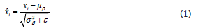
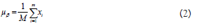
We compute the μ_β and σ_βover each mini batch β, during preparation, where

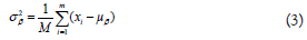
To consider putting the scale factor of zero, we fixed ε to a small tangible number. Using this equation, the activation with a batch normalization layer has a mean of zero and one variance. Batch normalization also provides the additional advantage of helping to stabilize instruction, allowing for a broad range of learning rates and regularisation capabilities.

Activation: We added a nonlinear activation function after the convolution sheet. An activation layer takes a W_input × H_input × D_input input volume and applies the activation function to it Figure 15. The output of an activation layer is often the same as the input dimension since the activation function is implemented element by element.

Figure 15: (a) Example image; (b) Final result matrix.

W_input=W_output, H_input=Houtput, D_input=D_output

Example-Consider the following image, which has had ReLU activation with the max (0, x) feature applied to it.

Pooling layers: The primary purpose of the pool layers is to gradually reduce the input volume’s spatial scale (width and height). We will reduce the number of parameters and computations in the network. Pooling also aids in reasonable control. In the pooling layer, we used the Max feature, that max pooling, with the pool size of F*S, that receptive field size into stride. The pooling process produces an output volume of W_output × H_output × D_output, where

W_output=((W_input-F)/S)+1

H_output=((H_input-F)/s)+1

D_output=D_input

Example-Consider a image of a mac pooling with pool size (2 × 2) and stride=1 added to it. We used two max-pooling layers of pool size 4 × 4 and stride=1 in work presented in CNN as described in Figure 16.

Figure 16: (a) Input image matrix b) Resultant matrix.

Flatten layer: This layer is used to flatten a three-dimensional matrix into a one-dimensional matrix. The array size obtained in the presented work is 6272 after flattening the sheet.

Dense layer: Dense is a unit of production. We have a binary problem in identifying brain tumors; it is entirely associated with one neuron with sigmoid activation. If the dense output is 1, the MRI is tumorous. If the lush production is 0, the MRI is not tumorous.

Fully connected layer: After extracting the features, we need to categorize the data into multiple classes, which we can achieve with a Fully Connected (FC) neural net. We may also use a traditional classifier like SVM instead of fully linked layers. However, we usually add FC layers to make the model trainable from beginning to finish. The fully connected layers develop a (potentially nonlinear) function between the high-level characteristics provided by the convolutional layers as an output using the sigmoid layer.

VGG-16 architecture using fast AI

Fast AI is a Python library that aims to make deep neural network training easy, scalable, fast, and accurate. As our base model for transfer learning, we chose the VGG 16 architecture. Upon request, the qualified architecture was downloaded and saved locally using the Fast AI API. Grampurohit, et al. “Brain tumor detection using deep learning models.” [24]. Two characteristics distinguish the VGG family of Convolutional Neural Networks-

The network’s convolution layers all use 3 × 3 filters.

We stacked several convolutions+ReLU layer sets until adding a pool function (the number of consecutive convolution layers+ RELU layers usually rises when we go deeper.

Instead of many hyper-parameters, VGG16 is based on making 3 × 3 filter convolution layers with a stride one and still uses the same padding and max pool layer of 2 × 2 filter stride 2. Throughout the design, the convolution and max pool layers are structured similarly. It has two Fully Connected layers (FC) at the top, followed by a softmax for output [25]. The 16 layer in VGG16 relates to the fact that it has 16 layers of different weights. This network is very vast, with approximately 138 million (approx.) parameters. We did not use the transfer learning methodology in the presented work; instead, we designed the VGG-16 architecture and made the required improvements to improve accuracy as shown in Figure 17.

Figure 17: VGG16 architecture.

Dataset and evaluation metrics

A total of 1500 benign and malignant brain tumor pictures are included in the suggested system, and the dataset con-tains 3060 T1-weighted contrast-magnified images of various malignancies.

Br35H is a binary tumor classifier. It includes image-based data. The Nr35H dataset is a standard dataset on which many deep learning techniques algorithms are compared on the same dataset [26]. On this dataset, the performance of CNN and VGG16 is 99.04% validation accuracy and 96.29%, respectively. This dataset comprises the images as well as the JPEG files. This dataset is also standard, and it has been compared to several other tumor detection algorithms. A sample of the two different images from our database is shown in Figure 18. To identify the images in this thesis, who will handle the entire database images with various image processing algorithms combined with CNN [27].

Figure 18: Sample of dataset combination with tumor and non tumor.

Because deep learning learns characteristics automatically, a large dataset is required. This dataset contains around 70% images for training. Each category is concerned with a particular point of view of the creatures, such as side view, back view, and front view. Testing data for the needed class is gathered from the Br35H dataset for evaluation [28,29].

Metrices evaluation

The Dataset is separated between 70% training, 15% validation, and 15% test sets using training and validation data, producing accuracy and loss graphs [30]. A classification report is prepared using the weighted average of precision, and precision, sometimes known as a Positive Predictive value (PPP), is a term used to describe the ability to remember something. Sensitivity, also known as Recall, is two other commonly used measures for segmentation accuracy. They are both based on the Confusion matrix, a 2*2 matrix (in the case of binary classification). Precision is calculated as follows-

Where TP=Total Positive and FP=False Positive, which calculates the proportion of true positives in the context of all optimistic predictions. Sensitivity is defined as the percentage of TP in the context of all true positives and is calculated as-

Where TP=Total Positive and FN=False Negative, which corresponds to the Total Positive Rate (TPR) and accuracy, computed as-

Will alone be used by the tumor segmentation. This metric is unsuitable for evaluating brain tumor detection, which is a very unbalanced task because negatives are far more than the number of positives. Accuracy is always highly valued in this environment.

Tool used

We used various software and hardware tools to carry out the proposed work, which is discussed further below-

Deep learning framework: Pytorch is a deep learning library that is open source and built on the torch library. It was created using CUDA, Python, and C++. In 2016, Facebook Inc.’s artificial intelligence teams produced the open-source application. Tensor computation and functional deep neural networks are two of PyTorch’s most unique capabilities. Tensors in programming differ from mathematical tensors in that a multidimensional array is used as a data structure. Tensors are used to implement these multidimensional arrays in Pytorch. On the other hand, these tensors support parallel computation via the CUDA parallel computation library.

Environment setup

We used the following environment for training our Neural Network architecture-

Software specification:

Operating systems: Windows 10

Python version: 3.8

Pytorch version: Pytorch 1.9.0

Python library: Opencv, numpy, pandas, matplot, cv2 etc.

Hardware specification:

CPU: 12v CPU

GPU: 14 GB Nvidia Tesla K40

RAM: 32 GB

Results and Discussion

Performance analysis

A comparison of our proposed deep learning-based classification models using the same dataset. The discrepancy in the accuracy is related to the dataset and these visuals-some differences in image parameters, illumination, sharpness, resolution, etc., all impact the results. One thing to remember is that the technique must be indicated. The total accuracy rate is obtained by adding the accuracy of each group in the confusion matrix and dividing it by the total of classes in the validation set is 99.00%. We reached 99.00 percent accuracy with CNN and 96.29 percent accuracy with VGG16.

Table 1 illustrates the accuracy of 99.04%, with 99.00% validation accuracy, a loss of 0.0358, and a validation loss of 0.0296. At the 11^th epoch of the preparation, this consistency was reached. According to this accuracy, the CNN with image size 240*240 and the cancerous brain database has the maximum validation accuracy rate of 99.00%. Furthermore, patient per image accuracy begins to be consistent, implying consistent predictions across patient photos. There’s a chance the test set is made up mainly of one class, and our model is biased in that direction, predicting the same class for such a majority of the inputs. To demonstrate that the test set is unbiased and that our model does not indicate the same grade for all intakes.

Table 1: Accuracy of CNN model.

In Figure 19, we plotted the loss graphs for the validation and training datasets. The loss plot shows that as the number of epochs increased, the training loss decreased while the validation loss increased and decreased. From the validation loss graph, we can see that we did not settle for local minima for validation loss and instead trained further. Validation loss increases while training loss decreases, resulting in overfitting. Because both the training and validation losses are reduced before converging, we conclude that overfitting does not occur. That shows that both validation and training accuracy are rising simultaneously. Overfitting occurs when the validation accuracy decreases at the expense of increasing training accuracy. Figure 20 illustrates the prediction of binary tumor classification using CNN.

Figure 19: History of accuracy and history of loss on training.

Figure 20: Prediction of tumor classification using CNN.

Table 2, illustrates the optimal platform only at the 8^th epoch, which offers a 92.20 percent accuracy rate and 96.29 percent validation data. Although the accuracy rate was gradually increasing after the 8th epoch, accuracy was steadily declining. We plotted the loss graphs for the validation and training datasets in Figure 21. As the number of epochs increased, the training loss decreased while the validation loss increased and decreased. Validation loss rises while learning loss falls, resulting in overfitting. We conclude that overfitting does not occur because both the training and validation losses are reduced before convergence. We also plotted the accuracy plot in Figure 21, which shows that both validation and training accuracy are increasing simultaneously. Figure 22 shows the results of binary tumor classification using VGG16.

Table 2: The original scale is used for all values.

Figure 21: History of accuracy and history of loss on training.

Figure 22: Simulation of tumor classification using VGG16.

Performance comparision

Several hyper-parameters are optimized to maximize predictive performance, and the system is instead validated. After acquiring better accuracy findings on a dataset of tumor pictures and distinct groups that have been identified, a comparative study was conducted between the suggested technique and past research, indicating the performance and high reliability of the research approach. In Table 3, the results produced using this method are compared to those obtained utilizing recently published articles and compares the suggested techniques to other research similar to ours. That also demonstrates the limitations of the associated study. Furthermore, and most significantly, it’s been asserted that the prediction accuracy in our research seems to be the best compared to various similar significant findings, as in the table below.

Table 3: Result comparison with state-of-art techniques.

Conclusion

We describe a novel CNN and VGG16 model for classifying brain cancers. As input, we used all pictures from an MRI dataset covering various types of cancers such as (Glioma, Meningioma, and Pituitary). The malignancies were pre-processed and segmented. CNN’s are cutting-edge in image recognition, and incorporating use in the healthcare profession enhances present patient-diagnosis techniques. CNN’s designed to detect tumor kinds in cerebrum images significantly boost recognition rate and lays the groundwork for incorporating deep learning into medicine. However, neural networks use a more generalized approach that requires essentially a visual to determine cerebrum tumor forms. Besides, this precision per person parameter stayed constant with the per imagery attenuation coefficients, implying that the neuron consistently produces patient imagery forecasts. The major challenge in imaging and pre-processing techniques is the computational complexity of handling multiple MR image modalities in an equal time frame. Our study achieved a fantastic outcome for the enhanced dataset. Its analysis revealed that our research seems to have a high accuracy of 99.00 percent, similar to several relevant studies.

Future Work

In terms of future work, we will explore various methods of expanding the set of data to expand the network’s prediction performance. A few of the transitions are to change the composition, and researchers might look at fine-tuning settings and applying motion to images during MR imaging scans for diagnosis. In the proposed study, deep neural networks such as CNN and VGG-16 get evaluated on MRI cerebrum representations. Both models yielded consistent results. However, VGG-16 needs more processing time and memory than CNN but produces acceptable results. Neural networks will play a significant role in statistical analysis in the coming days due to the vast amounts of data generated and processed by the medical industry. In the future, we will monitor the accuracy of the developed neural net, and the enhanced variants, on ongoing medical data. As a result, an exploration of natural 3D implementation rather than the slicewise approach could be one of the possible future directions in the progress of the local structure prediction algorithm.

References

1. Aneja D, Rawat TK. Fuzzy clustering algorithms for effective medical image segmentation. Int J Intell Syst App. 2013;5(11):55-61.

   [Crossref] [Google Scholar]

2. Kumar S, Dhir R, Chaurasia N. Brain tumor detection analysis using CNN: A review. IEEE. 2021:1061-1067.

   [Crossref] [Google Scholar]

3. Demirhan A, Toru M, Guler I. Segmentation of tumor and edema along with healthy tissues of brain using wavelets and neural networks. IEEE J Biomed Health Inform. 2014;19(4):1451-1458. [Crossref]

   [Google Scholar]

4. Joshi D, Goyal R. Review of tumor detection in brain MRI images. IEEE. 2019:27-28.

   [Crossref] [Google Scholar]

5. Deepak S, Ameer PM. Brain tumor classification using deep CNN features via transfer learning. Com Biol Med. 2019;111:103345.

   [Google Scholar]

6. Kunam AU, Sivagangai T, Sujatha ID. Brain tumor segmentation based on a various classification algorithm.

   [Google Scholar]

7. Pavithra M. Identification of pulmonary disease with chest x-ray data using CNN architecture. Turkish J Comp Mathematics Edu. 2021;12(12):2216-2221.

   [Google Scholar]

8. Saii M, Kraitem Z. Automatic brain tumor detection in MRI using image processing techniques. Biomed Stat Inform. 2017;2(2):73-76.

   [Crossref] [Google Scholar]

9. Siar M, Teshnehlab M. Brain tumor detection using deep neural network and machine learning algorithm. 2019 9^th International Conference on Computer and Knowledge Engineering (ICCKE). IEEE. 2019:363-368.

   [Crossref] [Google Scholar]

10. Sasikala S, Bharathi M, Sowmiya BR. Lung cancer detection and classification using deep CNN. Int J Eng Innov Technol Explor Eng. 2018;8(25):259-262.

    [Google Scholar]

11. Kiranmayee BV, Rajinikanth TV, Nagini S. Explorative data analytics of brain tumour data using R. 2017 Int Conf Curr Tre Computer Elect Electronics Commun. 2017:1182-1187.

    [Crossref] [Google Scholar]

12. Islam J, Zhang Y. A novel deep learning based multi-class classification method for alzheimer’s disease detection using brain MRI data. Brain Informatics. 2017:213-222.

    [Crossref] [Google Scholar]

13. Arya M, Sharma R. Brain tumor detection through MR images: A review of segmentation techniques. Int J Comput Appl. 2016;975:8887.

    [Google Scholar]

14. Krizhevsky A, Sutskever I, Hinton GE. Imagenet classification with deep convolutional neural networks. Adv Neural Inf Process Syst. 2012:25.

    [Google Scholar]

15. Pashaei A, Sajedi H, Jazayeri N. Brain tumor classification via convolutional neural network and extreme learning machines. 2018 8th International Conference on Computer and Knowledge Engineering (ICCKE) 2018;314-319.

    [Crossref] [Google Scholar]

16. Seetha J, Raja SS. Brain tumor classification using convolutional neural networks. Biomed Pharmacol. 2018;11(3):1457.

    [Crossref] [Google Scholar]

17. Ismael MR, Abdel-Qader I. Brain tumor classification via statistical features and back-propagation neural network. 2018 IEEE International Conference on Electro/Information Technology (EIT) 2018;0252-0257.

    [Crossref] [Google Scholar]

18. Gopal NN, Karnan M. Diagnose brain tumor through MRI using image processing clustering algorithms such as Fuzzy C Means along with intelligent optimization techniques. 2010 IEEE International Conference on Computational Intelligence and Computing Research 2010;1-4.

    [Crossref] [Google Scholar]

19. Sridhar D, Krishna IM. Brain tumor classification using discrete cosine transform and probabilistic neural network. 2013 International Conference on Signal Processing, Image Processing and Pattern Recognition 2013;92-96.

    [Crossref] [Google Scholar]

20. Srivastava N, Hinton G, Krizhevsky A, Sutskever I, Salakhutdinov R. Dropout: A simple way to prevent neural networks from overfitting. Mach Learn. 2014;15(1):1929-1958.

    [Crossref] [Google Scholar]

21. Devkota B, Alsadoon A, Prasad PW, Singh AK, Elchouemi A. Image segmentation for early stage brain tumor detection using mathematical morphological reconstruction. Procedia Comput Sci. 2018;125:115-123.

    [Crossref] [Google Scholar]

22. Pandav S. Brain tumor extraction using marker controlled watershed segmentation. Int J Eng Res Technol. 2014;2278-0181.

    [Google Scholar]

23. Bhandari A, Koppen J, Agzarian M. Convolutional neural networks for brain tumour segmentation. Insights Imaging. 2020;11:1-9.

    [Crossref] [Google Scholar]

24. Grampurohit S, Shalavadi V, Dhotargavi VR, Kudari M, Jolad S. Brain tumor detection using deep learning models. 2020 IEEE India Council International Subsections Conference (INDISCON) 2020:129-134. IEEE.

    [Crossref] [Google Scholar]

25. Yang G, Nawaz T, Barrick TR, Howe FA, Slabaugh G. Discrete wavelet transform-based whole-spectral and subspectral analysis for improved brain tumor clustering using single voxel MR spectroscopy. IEEE Trans Biomed Eng. 2015;62(12):2860-2866.

    [Crossref] [Google Scholar]

26. Sobhaninia Z, Rezaei S, Noroozi A, Ahmadi M, Zarrabi H, Karimi N, at al. Brain tumor segmentation using deep learning by type specific sorting of images. ArXiv. 2018.

    [Crossref] [Google Scholar]

27. Wu W, Li D, Du J, Gao X, Gu W, Zhao F, et al. An intelligent diagnosis method of brain MRI tumor segmentation using deep convolutional neural network and SVM algorithm. Comput Math Methods Med. 2020:6789306.

    [Crossref] [Google Scholar]

28. Kaur T, Gandhi TK. Automated brain image classification based on VGG-16 and transfer learning. 2019 International Conference on Information Technology (ICIT) 2019:94-98.

    [Crossref] [Google Scholar]

29. Jin KH, McCann MT, Froustey E, Unser M. Deep convolutional neural network for inverse problems in imaging. IEEE Trans Image Process. 2017;26(9):4509-4522.

    [Crossref] [Google Scholar]

30. Badza MM, Barjaktarovic MC. Classification of brain tumors from MRI images using a convolutional neural network. Appl Sci. 2020;10(6):1999.

    [Crossref] [Google Scholar]