Journal of Stock & Forex Trading
Open Access
ISSN: 2168-9458
ISSN: 2168-9458
Review Article - (2018) Volume 6, Issue 1
The market refers to the S&P 500 index SPY, which is an important benchmark of US stock performance. The following problem is of great interest: is there any trading system that can “beat” the market consistently? Proponents of the random walk hypothesis (RWH) and efficient market hypothesis (EMH) assert that stocks take an unpredictable path, and that it is impossible for a trader to outperform the overall market in the long run because stocks always trade at their fair values on stock exchanges. Therefore, the buy and hold (BH) investor has the best strategy.
This paper showcases a website (GeometricWavelet.com) containing an explicit wavelet trading strategy (WT) that “beats” the market consistently, contradicting the above assertion. The data set of SPY historical prices is used to show that WT “beats” the market. This data set is then fitted with a Geometric Brownian motion (GBM). Simulation shows that WT always outperforms the fitted GBM eventually and has larger risk adjusted returns. The numbers generated show that BH’s performance is far inferior to WT’s in the long run.
<Keywords: Wavelets; Efficient market; Geometric Brownian motion
Many economists, financial analysts, researchers, traders, and people acquainted with modern business finance theories consider that trading commodities and stocks by any system of buying and selling to make a profit is an impossible task, as there is plenty of empirical evidence and statistics against the existence of such a strategy; traders who buy and sell frequently usually end up losing money. In addition, proponents of the random walk and efficient market hypotheses, considered to be cornerstones of modern finance theory and economics, assert that stocks take an unpredictable path and that it is impossible to outperform the overall market consistently because stocks always trade at their fair values on stock exchanges. Observing that most people lose money in stock market trading brings many to conclude that trading is purely a game of luck. This paper will show that trading commodities and stocks is, in reality, more a game of skill than of luck.
There is a large body of literature on the random walk and efficient market hypotheses [1-18]. The random walk theory became well known since the year 1973 when Malkiel [10] published his book “A Random Walk Down Wall Street”. The efficient market hypothesis evolved from the work of Fama [4-6]. Both the random walk and the efficient market hypotheses have a strong influence on economics, modern market finances, and stock market trading. There are daily articles in newspapers on trading and related topics. The list of references listed here is a tiny fraction of the actual amount available.
The paper contains three components: the manuscript, the website GeometricWavelet.com and relevant data displayed at:
https://iu.box.com/s/2x7x3xsj5qzfy2pyt2m23ovoa38fsifp
which will be referred to as the link in this paper.. The website and the link are integral parts of the paper and they are open to the public. The market is the Standard and Poor’s 500 SPY index, which represents a collection of 500 stocks of a diverse group of US companies and is a popular benchmark to measure US stock performance. The SPY historical data set displayed at the link lists the dates and corresponding adjusted closing prices of SPY from January 29th, 1993 to October 3rd, 2017. The share price of SPY has increased more than eight hundred percent during this period. The adjusted closing prices represent an accurate reflection of SPY’s performance. They take into account corporate actions such as stock splits and dividends. The data were downloaded on October 4th, 2017 from the Yahoo Finance website online. These prices may look different if they are downloaded on another day. A date of the year will often be displayed in the same style of the SPY data set. For example, January 29th, 1993 is written as 1/29/1993 or 1/29/93.
Trading by WT is done through a brokerage which must satisfy certain conditions (stated in Sections 1 and 2) regarding commissions, margin interest rates and some other rules. The conditions are satisfied if the brokerage charges reasonable commissions, margin interest rates, and allows traders to use a margin loan at 2:1 leverage. Interactive Brokers (IB) is an example of such a brokerage. The commission charged by IB is $1.00 if the number of shares per trade is 200 or less; it is $0.005 per share if a trade involves more shares. The trader (WT) is an occasional trader who sells or buys SPY shares about once every few weeks. All money referred to is in US dollars.
The only stock traded is the S&P 500 index SPY. The trader enters the date and price of a share of SPY on the day she starts trading and on each trading day thereafter. The website contains a computer program which processes the information, and then tells WT whether to buy, sell or hold on each day of trading. The exact number of shares to trade is also specified on each day. Operating the website does not require any practice or skill on the part of the user. The paper is organized as follows:
Section 2 presents the website (also denoted by WT) and gives instructions for users. A lot of effort on my part has been devoted to make the website user friendly. Section 3 is devoted to show that WT “beats” the market in the long run based on the SPY historical data.
A Geometric Brownian motion (GBM) is fitted to the historical SPY data in Section 4. GBM is employed in the Black-Scholes model and is a very popular model for stock market prices. GBM is also known as exponential Brownian motion. GBM is always positive and tends to infinity with probability 1 if the drift parameter is positive. In addition, GBM is a Markov process, which means that all information on past historical prices is incorporated in the current price. The general belief is that it is impossible to “beat” a GBM since technical analysis of historical prices is useless in predicting future period. In Section 5, the fitted GBM is employed to generate simulated SPY data. The numbers generated by the website using the simulated data clearly show that the performance of BH is far inferior to WT’s in the long run. This result is quite surprising since it is now generally accepted among traders and academicians that the market is unbeatable and the buy and hold (BH) strategy is the best.
Section 6 presents the computation of the Sharpe Ratios of WT in the simulations. The calculations show that WT has higher risk-adjusted returns than BH.
My main objective is to find a winning strategy for a trader and not to debunk the random walk and efficient market hypotheses. However, the numbers produced by the website clearly show that the assertion that it is not possible to outperform a GBM or the market consistently is false. Even if past price and volume data have no relationship with the future direction of security prices, it is incorrect to conclude that excess returns cannot be earned by technical analysis.
Section 7 discusses the results of the paper and some other relevant issues. The main idea behind the strategy used by WT to “beat” the market is also explained in this section.
This section describes in detail what the website is about. Assume that both WT and WH use the same brokerage and the following assumptions are satisfied:
Assumption 1: WT is allowed a 2:1 margin leverage. The brokerage charges an interest rate no higher than 4% per year and collects interest daily (compounded once a day).
Assumption 2: The brokerage checks WT’s margin every day (usually around 4.00 pm) before closing time.
Assumption 3: The brokerage charges a commission equal to .04 percent of the cost of a transaction.
The author will now show why charging a commission which varies with the cost of the transaction as in assumption 3 is quite reasonable. Currently Interactive Brokers charges $1.00 for a trade with 200 shares or less. Later on, the paper contains discussions on future trades which can be many years ahead. How much will Interactive Brokers charge for commission for a trade of 200 shares of SPY, say, 30 or 40 years from now when the price of SPY may be in the thousands? It will be much more than one dollar. Thus 30 years from now, if a trader makes a trade of 200 shares of SPY, say, at $3,000.00 a share, the brokerage will charge a commission of $240.00.
Click on http://www.GeometricWavelet.com and the screen shows:
Welcome to GeometricWavelet.com
Run Geometric Wavelet Trading.
Click on “Run Geometric Wavelet Trading”, and then on “Enter Data” on the next page. Enter the date and price of SPY for each day of trading. The date needs to have two digits for the month, two digits for the day and four digits for the year. You can either type in the data or copy and paste it on the screen. If you choose to paste in the data, then you may need to format the “dates” column to make sure that there are four digits for the year as shown in Table 1.
| Dates | Price |
|---|---|
| 3/9/2009 | 56.88 |
| 3/10/2009 | 60.27 |
| 3/11/2009 | 60.66 |
| 3/12/2009 | 63.05 |
| 3/13/2009 | 63.54 |
| 3/16/2009 | 63.35 |
| 3/17/2009 | 65.29 |
| 3/18/2009 | 66.75 |
| 3/19/2009 | 65.92 |
| 3/20/2009 | 64.52 |
| 3/23/2009 | 69.15 |
| 3/24/2009 | 67.79 |
| 3/25/2009 | 68.51 |
| 3/26/2009 | 69.9 |
| 3/27/2009 | 68.64 |
| 3/30/2009 | 66.27 |
Table 1: Trading dates with share prices.
Let us start with an example. Consider the following set of data, which lists the price of SPY from 3/9/2009 to 3/30/2009.
After you enter the data, click on “Generate Table” and then wait for sometime for the website to process the information. The outputs are the Excel files: result.csv, result-no-zeros.csv and result.xlsx. They can be downloaded and opened in your computer. Result.csv is a text file which can be opened with a text editor but no text formatting can be done with this file. Result-no-zeros.csv is the same as result.csv with days of no trading deleted and result.xlsx contains the same information as result.csv but looks nicer. The output files and the data set above are displayed in the folder Exhibit 1 at the link. Please check to make sure that the output files that you obtain are the same as the files in Exhibit 1. Observe that WT is programmed to always buy 1,000 shares on the first day of trading.
If you type in a large set of data, then it is a good idea to save what you type in a text or Excel file for your record. If you mistype and then click on “Generate Table”, the whole data that you have entered may disappear. In case this happens, you still have a record of what you have typed, you can copy and paste your data back onto the computer screen, correct the mistype, and then repeat the process. The website does not hold any data for you after you logout.
The information contained in result.csv will now explained in detail. The first three columns list respectively the trading dates, share prices at which trades are made and the numbers of shares traded. A positive number for the shares in the third column means a “buy” and a negative one means a “sell”. A user of the website with the sole purpose of trading only needs to use the first three columns. The rest of the paper is to prove to the reader that WT always “beats” the market in the long run.
The fourth column lists the commissions charged by the brokerage for each trade. In result.csv, on 3/20/2009, WT buys 287 shares at the price of $64.52, she has to pay a commission of $7.41, which is much higher than the actual amount charged by Interactive Brokers or Scottrade.
The fifth column (CumCom) lists cumulative commissions, which are total commissions paid up to the trading day. For example, on 3/23/2009, after she sold 270 shares at the price of $69.15 a share, she has paid a commission of $22.75+$7.41+$7.47, which equals $37.63.
The sixth column (Cost) lists the cost of each trade which equals the number of shares traded multiplied by the share price. You have to pay the brokerage if it is a positive number and you get back cash if it is a negative number. A positive number for cost indicates a buy and a negative number indicates a sell.
The seventh column (CumCost) lists the cumulative cost paid by the trader. For example, after the fourth transaction is made on 3/30/2009, the trader’s cumulative cost is obtained by adding the four numbers on the sixth column, which equals $80,318.86.
The eighth column (CumShares) lists the total number of shares held by the trader after each trade. Note that after the fourth trade was carried out on 3/30/2009, the trader has a total of shares equal to 1,373, which is the sum of all numbers in Column 3 (Shares).
The ninth column (MV) lists the market value of the trader on each trading day. The market value (MV) is computed by multiplying the cumulative number of shares of the trader by the corresponding price.
Before going on to explain the rest of the columns in result.csv, the author needs to discuss some important aspects of stock market trading with a brokerage and the actions of WT and BH.
Margin
Buying on margin means borrowing money from the brokerage to buy stocks. The collateral for the borrowed funds is the stocks and cash in the investor’s account. Before buying on margin, an investor needs to open a margin account with the brokerage. Maintenance margin refers to the minimum amount of money that must exist in the account before the brokerage forces the investor to deposit more money.
In the United States, the Federal Reserve Board regulates the amount of margin that an investor must pay for a security. An investor is required to fund at least 50% of a security’s purchase price with cash. She may borrow the remaining 50% from a broker or a dealer.
A comparison of the performance of the trader (WT) versus the buy and hold (BH) investor will be made later on. Assume that both WT and BH have brokerage accounts at the same brokerage. Their actions are as described below.
Wavelet trading (WT)
She buys 1,000 shares of SPY on the first day of trading. She may use margin to buy additional shares according to the rules set up by the brokerage.
Buying and holding (BH)
The buy and hold investor takes the same action as WT on the first day of trading and makes no other trades from there on.
Note that the actions of WT and BH are identical on the first day of trading.
Next, the author will explain what the variable “cash” means. Cash is positive if the trader has surplus money in her account and negative if she owes the brokerage money. Assume that the brokerage charges 4% margin interest per year and that interest are compounded daily. Assume also that the brokerage does not pay WT any interest in case she has surplus cash in her account.
Cash
The amount of cash in BH’s account is always zero since all of BH’s money is in stocks. The amount of cash in WT’s account varies and is rather complicated to figure out. If she buys on margin and owes the brokerage money, the cash amount is a negative number. She has to pay interest to the brokerage on the money that she owes. The “Cash” variable of WT is zero between the day 3/9/2009 until 3/20/2009 when she bought on margin 287 shares at the price of $64.52 a share. The cost is 287×$64.52, which equals $18,517.24. Her cash after she bought 287 shares is -$18,524.65 which covers the $7.41 commission and the cost of the 287 shares. The negative sign indicates that she owed money after making this trade and she had to pay interest on this amount while she kept it. The formula for computing interest compounded every day is:
Int=A [1+(0.04/360))N-1],
where A and N are respectively the amount of money borrowed and the number of days that it is held.
Her next trade was a “sell” of 270 shares made on 3/23/2009 at the price of $69.15 a share. She has to pay $7.47 in commission and $18,670.50 for the cost of the shares. She now owes the interest on the $18,524.65 that she borrowed on 3/20/2009. This period is three days long and the interest is
Int=$18,524.65[(1.000111)3-1]=$6.18.
After the third transaction, her cash is -$18524.65+$18670.50-$7.47- $6.18, which equals $132.20. Her fourth trade occurred on 3/30/2009, when she bought 356 shares at the price of $66.27 a share. She earned no interest with her surplus cash. Her cash is now -$23,592.12-$9.44+ $132.20=-$23,469.36.
Account balance
The account balance of WT is the value of her account, which is equal to the sum of her MV and Cash. The account balance of BH is just equal to BH’s market value, which equals 1,000 times the share price.
Buying power
This is the money still available for WT to buy additional shares. She can borrow from the brokerage up to 100% of her net liquidation amount, which is her account balance. Hence, her current buying power equals:
Account Balance+Cash=MV+Cash+Cash=MV+2 Cash.
WT return
On the first day of trading, WT buys 1,000 shares at the price of $56.88 a share. She has to pay $56,880 for the cost of the 1,000 shares and $22.75 in commission fee. WT’s return on the first day of trading is -$22.75. On any other day, her return equals:
Account Balance -$56,880-$22.75.
On the last day of trading, her return is $67,519.35-$56,880-$22.75= $10,616.6.
BH return
At any given share price, BH’s return is computed as follows
BH’s Return=1,000 × Price-$56, 880-$22.75.
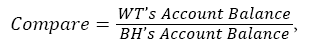
Compare: The variable Compare is defined as:
with
WT’s Account Balance=WT’s Return+$56,880+$22.75,
BH’s Account Balance=$1,000 × Price.
The account balances of both WT and BH are positive numbers while their returns can be any number. A value of Compare greater than 1 indicates that WT does better than BH and a value less than 1 indicates otherwise.
The tenth column (Cash) lists the amount of cash that WT has.
The eleventh column (buying Power) lists the amount money that WT can still use to buy.
The twelfth column (L) lists the interests that WT pays.
The thirteenth column (M) shows the account balance of WT.
The fourteenth and fifteenth columns list, respectively, the returns of WT and BH.
The sixteenth column (Compare) lists the daily values of the variable Compare.
Note that Compare is always a positive number.
Since the year 2009 to the present time, all the conditions regarding margin interest, margin leverage and commissions are satisfied for an owner of a brokerage account at Interactive Brokers. Interactive Brokers was established in 1993 and is the largest US. electronic brokerage firm by number of daily average revenue trades. Currently, Interactive Brokers charges about the lowest commissions and margin interest rates among the largest several brokerages. Margin interest rate at Interactive Brokers fell way below 4 percent since 2009. An owner of a memorandum account with a minimum balance of $25,000 can use a 2:1 margin to buy additional shares. A trader with more than $100,000 can open a special memorandum account, which allows a 2.25:1 margin.
Exhibit 2 at the link contains the details of the trades of WT with different starting dates during the period 2009-2016. During this period, interest rates are low in general and margin interest rates charged by Interactive Brokers are below three percent. Note that Compare is always greater than 1 by 10/3/2017, which is the last day of trading. For example, if WT started trading on 2/16/10, then compare would be 1.22 by 10/3/17, which means that her account balance is 1.22 times the account balance of BH by this date. Observe also that WT never gets a margin call since the numbers on Column K are always positive.
The equation for a geometric Brownian motion (GBM) is given by:
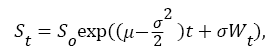
where Wt is standard Brownian motion. Here, St is the value of GBM at time t and S0 is the initial value. The parameters -∞<μ<∞ and σ>0 are constants. GBM serves as an important example of a stochastic process satisfying a stochastic differential equation.
The mean and variance of St are:
E(St)=S0 exp(μt)
Var(St)=(S0)2 exp (2μt) exp (σ2t)-1.
Let Xt=log St-log St-1. Then,
Xt=μ-(σ2/2) +σ(Wt-Wt-1),
which is normally distributed with mean μ-(σ2/2) and standard deviation σ. A total of 6,215 values of Xt are obtained from the SPY historical data set at the link. Using these values, estimates of the drift parameter μ-(σ2/2) and standard deviation are, respectively, 0.000356 and 0.011617. These estimates are, respectively, the sample mean and sample standard deviation of 6,215 observations of Xt’s. The parameter μ is estimated to be 0.000424.
Since the drift parameter μ-(σ2/2) is positive, St tends to infinity with probability 1. This fits well with SPY which has been rising fairly steadily with time. The reader is referred to Oksendal [11] and Ross [13] for more information on GBM.
In all the simulations to be discussed in this section, the day 10/03/2017 is set to be t0 and the initial price S0 is set equal to 252.86, which is the price of SPY on 10/3/2017. The equation for the geometric Brownian motion obtained is
St=252.86 exp (0.000356t+0.011617Wt).
A simulation to evaluate and compare the performances of WT and BH can be carried out as follows.
1. Click on “Run Geometric Wavelet Trading” and then on “Random Data” at the website. Click on “Generate Data” and wait for a couple of minutes for the website to generate random daily prices of St for a total of 300 years, starting on 10/3/2017 and ending on 7/23/2317. These dates will be referred to, respectively, as the first day and last day of trading.
2. Click on “Generate Table” and then wait about five to ten minutes for the website to generate the files result.csv, result-no-zeros.csv and result.xlsx.
Three hundred years of daily prices are about the maximum amount of data that the website can handle. The results of 1,000 simulations are posted in the folder Results at the link. They are labelled as result-0000.csv to result-0999.csv. You may need to click on “Name” at the upper left corner of the screen to arrange the files in the right order.
Let us look at result-0000.csv as an example. On the first day of trading, both WT and BH buy 1,000 shares of SPY at $252.86 a share for a total cost of $252,860. On this day, they have the same account balances and Compare is equal to 1. The buying power of WT is also $252,860 since WT does not borrow any money yet. On the last day of trading, Compare is 722.89 which means that WT’s account balance is as big as 722.89 times BH’s account balance.
In all of the 1,000 cases, Compare is greater than 1 by the last day of trading. Observe that WT never gets a margin call since the numbers on Column K are always positive. The simulations show that WT always outperforms BH, and consequently, the market in the long run.
Does WT earn much higher risk-adjusted returns than BH? This question can be answered by finding their Sharpe ratios. The Sharpe Ratio (denoted by SR) is widely used for risk-adjusted returns and can be computed using the formula:
SR=(Average Rate of Returns Risk-free Rate)/σ(Rate of Returns),
where σ denotes the standard deviation.
Since the risk-free rates from 10/3/2017 to 7/23/2317 are not known, the rates of returns of WT are bench-marked against the realized values of SPY instead. The ratio computed is called the ex-post Sharpe ratio. The computation of SR is carried out for result-0000.csv and displayed in the file Sharpe Ratio.xlsx at the link. To view this file, you may have to download it to your computer and use Excel to open it. The market has SR equal to zero while WT has SR equal to 0.03. Thus WT has higher risk-adjusted returns than BH.
The file stats.csv at the link shows some important statistics derived from the 1,000 simulations done. The first column of stats.csv lists the names of the files.
The second column of stats.csv lists the values of Compare on the last day of trading for each simulation. They are all greater than 1, with mean equal to 391.42 and median equal to 158.01. The largest is 22,950.88 from result-0745.csv and the smallest is 2.16 from result-0507. This shows that WT has an account balance much higher than BH by the last day of trading. Consequently, WT always “beats” the market overwhelmingly in the long run.
The third column (MinComp) of stats.csv shows the minimum value of Compare among the 109,501 numbers displayed for each file. The smallest number on the third column is 0.37 from result-0203. Compare reaches this number on 5/15/2066. On this date the account balance of WT is equal to 37 percent of BH’s account balance. However, WT manages to recover later on and her account balance is as large as 115.94 times BH’s by the last day of trading. The mean and median of MinComp are, respectively, equal to 0.85 and 0.89.
The fourth column (MaxComp) of stats.csv displays the maximum value of Compare among the 109,501 numbers displayed. This maximum is the “all time high” among all the 109,501 numbers of Compare.
The fifth column (T1) of stats.csv shows the numbers of days it takes to “beat” the market. On average, it takes 8,276 days (22.67 years) to outperform the market. However, the median of T1 is 3,548 days (9.72 years). This indicates that T1 has a heavy-tailed distribution skewed to the right.
The sixth column (T2) of stats.csv presents the number of days for Compare to hit 2. Here T2 is waiting time for the account balance of WT to be twice as much as BH’s. The average and the median of T2 are, respectively, 15,969 days (43.75 years) and 12,508 days (34.27 years).
The seventh column of stats.csv lists the 1,000 ex-post Sharpe ratios of the simulations. Note that they are all positive, indicating that WT always has higher risk-adjusted returns than BH in the long run.
The rest of the section is to discuss some other relevant issues.
1. A trader using WT should check the price of SPY daily. She is required to buy, sell or hold according to the guidance of WT.
2. Suppose WT advises a trader to buy or sell 200 shares at some price. The trader may not be able to buy or sell 200 shares at exactly the price recommended since the price of the stock might have changed by a small amount by the time she actually buys or sells. Buying or selling at prices approximately equal to the prices recommended by WT would not affect the trader’s overall return much.
3. What if the user of WT trades more frequently, for example, every hour of the day? Trading here means she enters the date, share price and take the action recommended. This will probably increase her return. It would be interesting to see how WT performs with continuous data. I do not have a definite answer to the question at this time.
4. A trader can also start with an amount of shares different than 1,000. Suppose she can afford to buy only 500 shares to start with. Then she should cut down her trades to be one-half of WT.
5. What would the results be if a different stochastic process (probably heavy tailed) is fitted to the SPY historical data? They might change somewhat but not be enough to affect the conclusion that WT outperforms the market in the long run. The fitted process must have an increasing trend.
6. The Black-Scholes model assumes that it is possible to borrow any amount of money at the risk-free rate, and trades do not incur any fees. If this is the case, WT can increase her return considerably.
7. A reader can easily replicate the simulations done in the paper by using the website.
WT’s main idea is to use margin loans from the brokerage to gradually increase her cumulative number of shares while avoiding margin calls. For example, in result-0000.csv, she starts with a buy of 1,000 shares. Her cumulative share on column H increases slowly and eventually reaches 1,013,265 by 2/3/2317. Note that her cash decreases significantly on many trading days when she borrows money to buy additional shares. Here the shares that she buys after the first day of trading are referred to as additional shares.
WT has to pay interests on the money borrowed on margin to buy additional shares and also has to pay extra commissions. But the sum of the latter expenses are much less than the gain due to increases in prices of the additional shares. By holding more shares than BH, she ends up with larger returns than BH.
Her main effort is in maintaining positive buying powers to avoid margin calls. Serial dependence of the observations, regressions, market timing, and prediction do not play any important role in her strategy. The important variables are interest rates, commissions, buying powers. Account balances and market prices.