Advanced Techniques in Biology & Medicine
Open Access
ISSN: 2379-1764
ISSN: 2379-1764
Research Article - (2015) Volume 3, Issue 3
Stem cells have the remarkable ability to cultivate itself into any kind of cell in the body at their early stage of growth. In some organs, such as the gut and bone marrow, stem cells regularly divide to repair and replace worn out or damaged tissues. The existing methodology for stem cell analysis image segmentation makes use of a morphological technique applied on the fluorescent cells so as to get a clear cut segmented image. For this the wavelet Otsu Curvelet paradigm is used in where the image or frame is filtered, Curvelet is used for better edge enhancement and Wavelet is used for multi-scale resolution. Segmentation using Otsu model, reduces the average weight of class variances from various pixels to provide an optimal threshold value. From the segmented image feature, vectors are obtained using Grey level co-occurrence matrix (GLCM) technique which plays a vital role in extracting the features in an image. However GLCM commonly extract the texture under single scale and single direction which does not provide the textural entities to its maximum extent. Hence for multi scale and multi-resolution, the segmented image is decomposed with NSCT and GLCM is applied. The set of feature vectors form finally the pattern matrix as the input to the artificial neural networks for their classification. Using neural network for pattern recognition, the network is trained by using the images of various healthy level images. Then using the trained network, the healthy nature of the test image is evaluated and the result is displayed in the form of percentage of healthiness of the given time series stem cell images. Hence this paper is highly motivated to analyse the healthy nature of stem cells.
Keywords: Stem cells, Grey level co-occurrence matrix (GLCM), Neural network
Pattern recognition is a machine learning process that emphasizes on the various discontinuities in data. It can also be stated as how machines differentiate the region of interest from the background. This is initially done by the classification of patterns either into supervised or unsupervised class based on the similarity or system designer. A well defined recognition system will have less variations in intra class and high variations in inter class.
Observations based on a set of samples known as training data serve to be an important feature in most of the recognition systems [1]. The accuracy and performance is improved with the application of artificial neural networks (ANN).
The nature of a stem cell is evaluated in three steps: segmentation, feature extraction and pattern recognition. Segmentation partitions the image into many segments based on the intensity making the image homogeneous thus providing a newer representation for better analysis. Secondly the feature extraction helps to discriminate the healthy cells from the cell image. Lastly the pattern recognition is done on the basis of feature vectors.
The Otsu algorithm [2] is one of the simple methods for image segmentation. Wavelet frames [3] resolves the restoration problems such as denoising, deblurring, etc., Multi-phase segmentation divides the image into many labels depending on the application. The region of interest (ROI) can be classified automatically using wavelet transform [4] by multi resolution analysis. For reconstructing the segmented image without any visual artifacts both ridgelet and curvelet transforms have been implemented [5]. They are not adaptive and found to be effective in piece wise images [6]. The curvelet transform is an extension of ridgelet and wavelet that operates on curves. It has significance in classifying the abnormal tissues and reducing the noise [7] Grey level quantization is used for classifying natural textures relating with cooccurrence ability [8]. Correlation analysis is performed on a set of statistics namely the contrast, entropy and correlation.
The non-subsampled Contourlet transform (NSCT) [9] is developed on the pyramidal and directional filter banks which gives shift invariant, multi-scale and multi direction image for decomposition. The input in pattern recognition is a set of data extracted by image processing algorithms [10]. It is the final step for interpreting any image. The complex data sets can be also processed by artificial neural networks which act as an intelligent technique [11]. This also overcomes the various challenges faced in bio-medical data such as stem cell images.
The artificial neural networks that are being evolved from biological neural systems work on the learning ability of the intelligent classifiers. It is a parallel processing system whose nodes are practiced for learning and decision-making. The nodes are able to perform elementary computations and learning is obtained by the varying weights that each node carries in order to connect with each other. ANN is widely used as classifiers in medical imaging [12,13]. The features extracted from an image are fed as input to ANN that calculates the weights in training data where the supervised classification is known and ANN is used for further classification of new data. ANN’s are used as a clustering method [14,15]. Major applications of ANN involve disease diagnosis such as liver cancer detection [16], detection of the outline of lungs in MRI [17], brain tumour classification [18], abnormal retinal classification [19]. The lung cancer detection uses fuzzy mean clustering algorithm [20]. This serves to be an efficient method for classifying the stem cells.
Hybrid fast woc segmentation
To obtain better segmentation results with reduced complexity when compared to previous algorithm, WOC (wavelet Otsu curvelet) method is incorporated and it is prescribed in the following flow diagram (Figure 1).
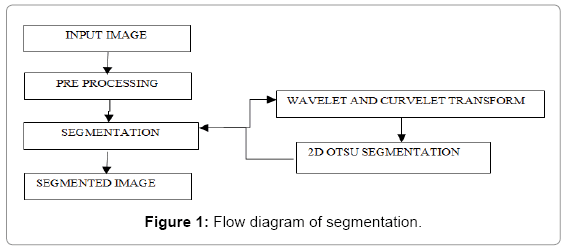
Figure 1: Flow diagram of segmentation.
The input stem cell image enhanced with anisotropic filtered image. It is used to diffuse the speckle noise present in the image. But due to degradation in the structure, it cannot sustain the resolution of the image. So wiener filtering is implemented to reduce the speckle noise as well as noise present in the edges without affecting the edge pixels. After pre-processing, segmentation is carried out by the combination of WOC (Wavelet, OTSU and Curvelet) technique. First wavelet transform is applied to solve point discontinuous problem. But it is affected by curve discontinuity, which is eliminated by using curvelet transform. And also gives better directionality to edges. The grey level distribution of pixels is utilized by histogram based OTSU algorithm. The optimal threshold vector is selected by using the average grey level distribution of their neighbourhood pixels.
Non sub-sampled contourlet transformation (NSCT) feature extraction
To efficiently approximate the images made of smooth regions separated by smooth boundaries, the contourlets transform form a multiresolution directional tight frame. It is implemented faster by Laplacian Pyramid Decomposition proceeded by directional filter banks applied on each band pass subbands. Even though the Contourlet transform has number of useful features and qualities, it has some blemishes. The nonsubsampled Contourlet transform (NSCT) was introduced mainly due to its shift invariance property.
In NSCT [21], the Laplacian Pyramid Decomposition present in Contourlet transform is replaced by a nonsubsampled pyramid filter to have the multiscale property and a nonsubsampled directional filter to have maximum directionality. The main prominent difference is that up-sampling and down-sampling are removed from both processes and are just only up-sampled. Though it avoids shift invariance issue it has problems with aliasing and directional filters.
Existing image enhancement methods amplify noises when they amplify weak edges since they cannot distinguish noises from weak edges. The nonsubsampled Contourlet transform provides not only multiresolution analysis, but also geometric and directional representation with time invariance. Since weak edges are geometric structures, while noises are not, we can use this geometric representation to distinguish them (Figure 2).
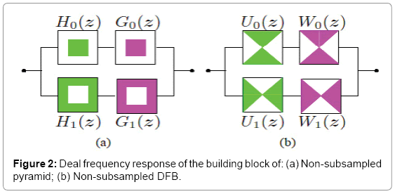
Figure 2: Deal frequency response of the building block of: (a) Non-subsampled pyramid; (b) Non-subsampled DFB.
Design of pattern recognition (Figure 3)
Pattern recognition classifies data based on either the prior knowledge or on statistical information extracted from patterns. Patterns are groups of observations defining points in multi dimensional space. The recognition system consists of sensor that gathers observations; a feature extraction mechanism that computes symbolic or numeric information from those observations; a classification scheme that describes observations relying on the extracted features. The classification scheme is based on the availability of set of patterns that have already been described. This set of patterns is termed as training set and the resulting learning strategy is characterized as supervised data. The classification follows statistical or syntactic or neural approach. Statistical recognition assumes that the patterns are generated by probabilistic system. Structural recognition is based on the structural inter relation of features. Neural recognition employs neural computing.
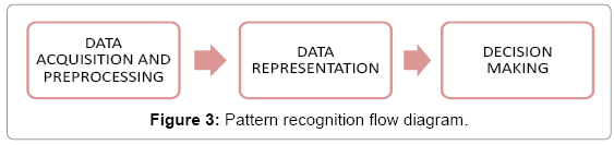
Figure 3: Pattern recognition flow diagram.
Artificial neural network: ANNs are computational mathematical model which got inspired by biological Neural Networks. These networks are generally presented as interconnected neurons to transmit messages with one another. These connection hold a weighted value which is altered based on prior knowledge, this makes the network adaptive to inputs and capable of learning. When an input is given the output is computed based on the present weights and then changes systematically based on the difference between the output and the target output and this end when the output value equals the target output.
Feed-forward, back-propagation ANN’s: The most commonly used structure for neural network has three layers as shown. The line between the nodes indicates the flow of information from one node to next. In particular networks the information flows only from input to output known as feed forward network in other types it may have intricate connections called feedback path. The input nodes are passive which means they cannot modify the data whereas the hidden and output layers are active. The value of the input node is duplicated and sent to all hidden nodes and this forms fully interconnected structure. The values entering the hidden nodes are multiplied by weights that are pre-determined in the program. The output of the hidden layer after summing and sigmoid function is duplicated as before and sent to output layer. The output nodes modify and combine data to give results (Figure 4).
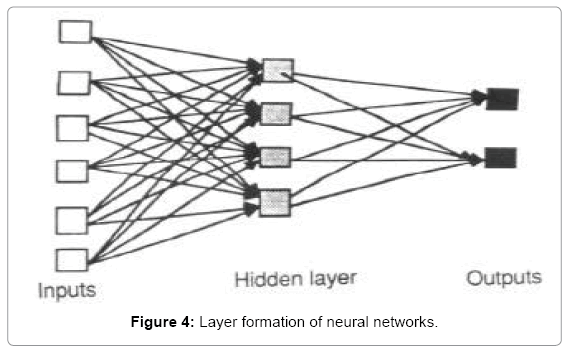
Figure 4: Layer formation of neural networks.
Determining the number of nodes in the input layer: The nodes input layer is equal to the number of columns in the data. In few neural networks an extra node is added to the input nodes as bias node. Thus the total nodes in the input layer are given as the input vector length plus one more neuron as bias node.
Determining the nodes in output layer: The number of nodes in the output layer is determined by the mode in which the neural network operates. There are two configuration modes namely machine mode that results in class label and regression mode that gives value. When NN acts as regressor signal node serves as an output layer and NN as classifier it has one node for every class label. Thus one output node will able to evaluate the nature of the stem cell in percentage.
Determination of hidden layers: The nodes size in the hidden layer is somewhere between the size of input and output layers. For better efficiency we set the number of nodes close to the input size so as to avoid difficulties in converging. As a rule the number of hidden layer nodes can also be fixed as the mean of the input and output neuron size.
Segmentation
The time-lapse image data of stem cells is chosen as an input image. Many experiments have been done for time lapse series image segmentation. Tracking and analysis of the morphological changes of cells are the challenging tasks in image processing. Stem cells are very powerful cells found in both humans and non-human animals. Stem cells are capable of dividing and renewing themselves for long periods. They are unspecialized cells which can give rise to specialized cell types and shown in Figure 4 (Figure 5).
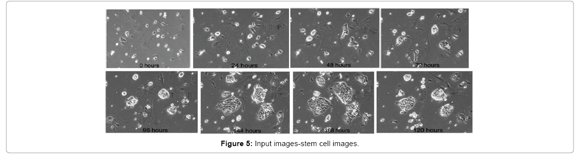
Figure 5: Input images-stem cell images.
Anisotropic diffusion filter analysis: Input images are given to anisotropic diffusion filter. The filter first diffuse the image because some speckle noise present in image, naturally speckle noise have circular and small in size. The diffusion technique helps to enhance that noise and remove it.
The output image is the result of the both the original image and the filter that works on the local content of the image. This shows that the anisotropic diffusion is non-linear and space variant transform of the original image. The output images of anisotropic filer shown in Figure.5. The main advantage of anisotropic filter is used to diminish noise in smooth regions and maintain edges to a higher extent. The problem is adjusting different parameters such as the number of iterations. Due to the degradation in fine structure, the resolution of the image is reduced. To prevent this degradation wiener filter is implemented in this technique (Figure 6).
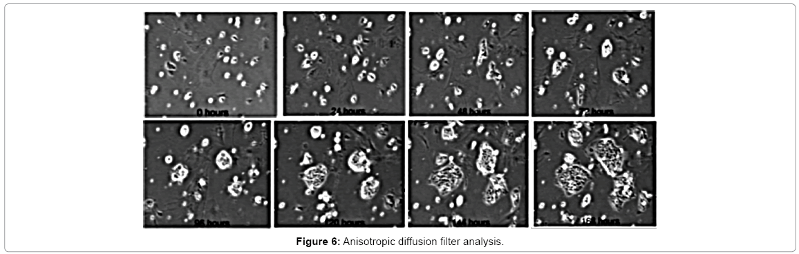
Figure 6: Anisotropic diffusion filter analysis.
Wiener filter analysis: Wiener filter is a linear filter that gets a linear assessment of an anticipated signal sequence from another related signal sequence. The main function of the wiener filter is to decrease the noise existing in an image by relating with the noiseless image. It is a mean square error optimal stationary filter that is used in images that are ruined by additive noise and blurring. It is applied in frequency domain because of the unfocussed optics and linear movement. Each pixel of a digital image signifies the intensity of an inert point in opposite of the camera. Unfortunately, due to camera misfocus and shutter speed, the given pixel will have an amalgam of intensities. The wiener filter is used to filter this corrupted signal. In wiener filter, one has the knowledge of the spectral properties of the original image and noise and performs linear time invariant so as to get the close to the original image. Wiener filter also used to removing speckle noise present in the images and also remove noise present in the edges. When compare output of anisotropic and wiener filters in term of PSNR (power signal to noise ratio) wiener filter has good PSNR value and output images shown in Figure 6 (Figure 7).
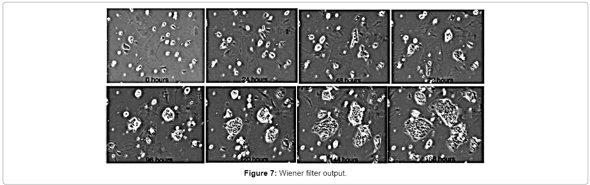
Figure 7: Wiener filter output.
Woc segmention analysis:
Algorthim:
1. I=Input Image.
2. Obtain the histogram values (h) of the image I.
3. Set the initial Threshold value:
Tin=Σ( h*total shades) / Σ h
4. Segment the image using Tin. This will produce two groups of pixels: C1 and C2.
5. Repeat step-3 to obtain the new threshold values for each class. (TC1 and TC2).
6. Compute the new threshold value:
T=(Tc1+Tc2)/2
7. Repeat the steps 3-6 until the difference in Tin successive iterations is not tends to zero
8. Now apply the Otsu method for the obtained threshold value for further segmentation process. (Figure 8)
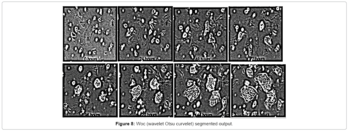
Figure 8: Woc (wavelet Otsu curvelet) segmented output.
Weiner output given to WOC (wavelet Otsu curvelet) segmentation, wavelet transform have multi scale property, curvelet have multiresolution property and Otsu segmentation is simplest segmentation process and execution time also less compared to other techniques. The wavelet based method try to separate signal from noise and not to degrade the signal during the de-noising process. Wavelet used as decomposition part in curvelet and histograms based threshold finding Otsu segmentation is used to obtain better segmentation results. Weiner filter helps in detecting the low frequency components present in the image. Hence the inner details of the image are getting, curvelet operates on the high frequency part of the image and helps in detecting the edges clearly. Finally segmentation is done by using a thresholding based on histogram using Otsu algorithm. In this technique the threshold is calculated based on the histogram of the image and the image is segmented. The region with uniform intensity gives rise to strong peaks in the histogram. And the histogram based threshold selection is good if the histogram peaks are tall, symmetric, and narrow and separated by deep valleys. The high homogeneity region produces low variance. The histogram based Otsu gives better results in salt and pepper noise and does not support Gaussian noise. But the combination of WOC method gives better segmentation output shown in Figure 8, for both salt and pepper and Gaussian noise.
Comparision analysis: The Table 1 illustrates comparison between anisotropic filter and Wiener filter. It gives the segmentation results comparison of WO and WOC method with precision, recall, and PSNR value. Anisotropic filter used to smooth the noise and it leads to also blur the edges. It dislocates the edges while arriving from finer to coarser scale. So the output error cannot be controlled as much. Due to this problem PSNR value of the anisotropic output is decreased. In the case of wiener filter, though it is scale invariant, it begins to exploit signal and the output error is controlled, PSNR value is maintained. Comparing anisotropic filter and wiener filter, the wiener filter has good PSNR value. After segmentation PSNR value increased because wavelet transform has noise removal characteristics. The discontinuity in lines or curves is eliminated by implementing wavelet transform. But it needs the more number of wavelet co-efficients to account edges through lines. The necessity of coefficient can be solved by optimal ridgelet in curvelet transform. Hence Wavelet OTSU segmentation is enhanced by integrating Wavelet, Curvelet and OTSU transforms and pointers to good precision, recall, and PSNR value (Table 1).
| INPUT MAGES(Stem Cell) | PREPROCESSING (PSNR) | WO–SEGMENTATION(Wavelet-OTSU) | WOC–SEGMENTATION(Wavelet-Curvelet-OTSU) | |||||||
|---|---|---|---|---|---|---|---|---|---|---|
| ANISOTROPIC FILTER | WIENER FILTER | P | R | PSNR | P | R | PSNR | |||
| 0 HOUR | 26.8004 | 35.4527 | 0.87897 | 0.910 | 59.7855 | 0.99945 | 1 | 65.19275 | ||
| 24 HOUR | 25.7344 | 35.1145 | 0.87805 | 0.910 | 54.1993 | 0.99897 | 1 | 59.78552 | ||
| 48 HOUR | 25.932 | 34.4389 | 0.87808 | 0.910 | 54.3113 | 0.99908 | 1 | 60.67717 | ||
| 72 HOUR | 26.9711 | 35.3818 | 0.87855 | 0.910 | 56.7726 | 0.99933 | 1 | 63.41392 | ||
| 96 HOUR | 25.185 | 33.524 | 0.87805 | 0.910 | 54.1993 | 0.99903 | 1 | 60.21991 | ||
| 120HOUR | 24.8863 | 32.4116 | 0.87787 | 0.910 | 53.4528 | 0.99905 | 1 | 60.44553 | ||
| 144HOUR | 23.8537 | 31.3342 | 0.87803 | 0.910 | 54.0886 | 0.99903 | 1 | 60.21991 | ||
| 168HOUR | 23.0605 | 31.2077 | 0.87800 | 0.910 | 53.97940 | 0.99908 | 1 | 60.67717 | ||
Table 1: Results analysis of filtering and segmentation process, where ‘P’ denotes Precision, ‘R’ denotes Recall and PSNR denotes Power Signal to Noise Ratio.
NSCT algorithm
1. Compute the NSCT of the input image for N levels.
2. Estimate the noise standard deviation of the input image.
3. For each level DFB,
(a) Estimate the noise variance.
(b) Compute the threshold and the amplifying ratio.
(c) At each pixel, compute the mean and the maximum magnitude of all directional subbands at this level, and classify it by (1) into strong edges, weak edges, or noises.
(d) For each directional sub band, use the nonlinear mapping function given in (2) to modify the NSCT coefficients according to the classification.
4. Reconstruct the enhanced image from the modified NSCT coefficients (Table 2).
| 0 hours | ||
| Feature Vector | GLCM | NSCT |
| ENERGY | 0.1163 | 0.8626 |
| AUTOCORRELATION | 4.2714 | 7.3460 |
| HOMOGENITY | 0.1742 | 3.0057 |
| CONTRAST | 0.0983 | 1.8875 |
| ENTROPY | 0.0937 | 0.6128 |
| DISSIMILARITY | 0.2787 | 0.9858 |
Table 2: Feature vector comparison between GLCM and NSCT for ‘0’ hour.
Table 2 illustrates the different feature parameters output comparison between GLCM and NSCT for stem cell input image at 0 hours. Because of multiscale, multidirectional process of NSCT, the feature parameter are extracted efficiently when compared with single scale, single directional GLCM.
Training and testing the ANN’s
In order to generate as many images as possible for training and testing the ANN, the 93 255 × 255 images were taken. These were separated into unhealthy (47), good (20) and healthy (16) images and these were given for training and testing. The flowchart in Figure 6 shows the steps to train and test ANNs with these images (Figure 9).
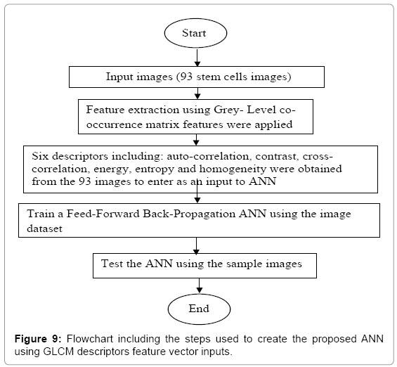
Figure 9: Flowchart including the steps used to create the proposed ANN using GLCM descriptors feature vector inputs.
STEP 1: Two matlab databases are created one for the input values and another for target values (Figure 10 and 11).
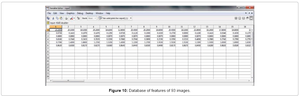
Figure 10: Database of features of 93 images.
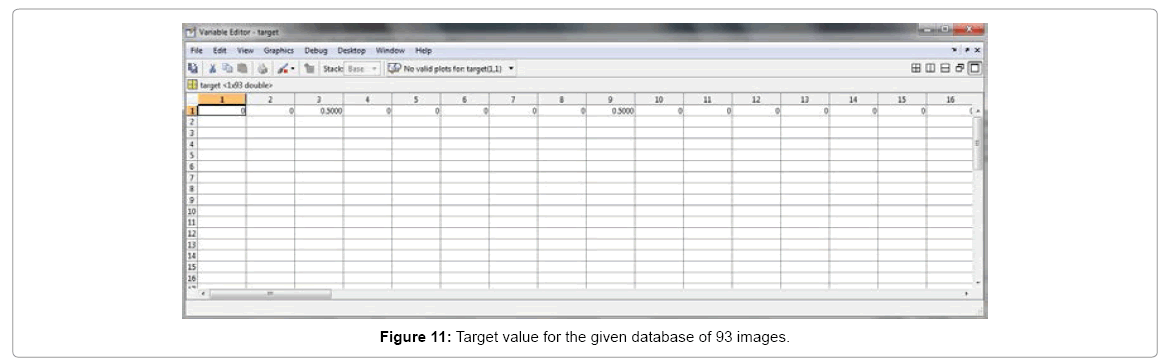
Figure 11: Target value for the given database of 93 images.
STEP 2: The features of the image for which the healthy nature is to be evaluated is given as the sample input (Figure 12).
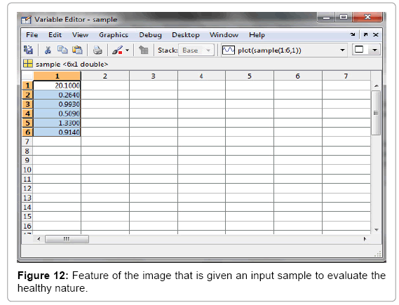
Figure 12: Feature of the image that is given an input sample to evaluate the healthy nature.
STEP 3: Open the neural network toolbox by typing ‘nntool’ in the command window then Network manger toolbox opens where the created database are imported (Figure 13 and 14).
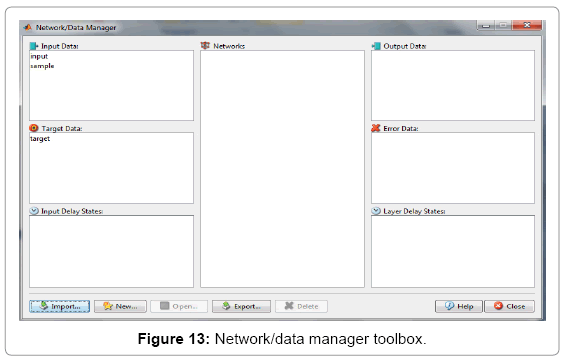
Figure 13: Network/data manager toolbox.
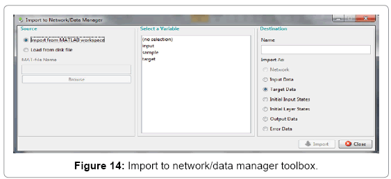
Figure 14: Import to network/data manager toolbox.
STEP 4: Click on the ‘new’ icon in the network/data manager toolbox to create a new neural network. In the Create Network or Data mention the name of the network, network type, input data, target data training functions, learning functions, number of layers, and number of neurons. Then click on ‘create’ icon (Figure 15).
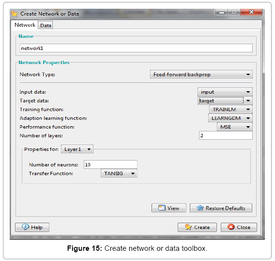
Figure 15: Create network or data toolbox.
STEP 5: In the network/data manager click on ‘network’ and open then the designed neural network opens. (Figure 16).
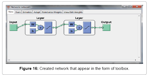
Figure 16: Created network that appear in the form of toolbox.
STEP 6: In the network toolbox click on train network and give input target and the training parameters (Figure 17 and 18).
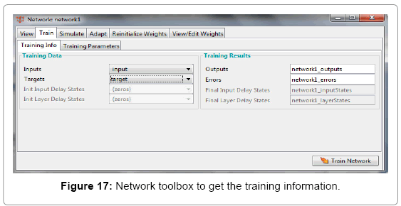
Figure 17: Network toolbox to get the training information.
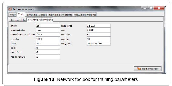
Figure 18: Network toolbox for training parameters.
STEP 7: Click on train network, the network is trained.
STEP 8: Click on simulate icon in the network toolbox then give input as the sample and click on simulate network (Figure 19).
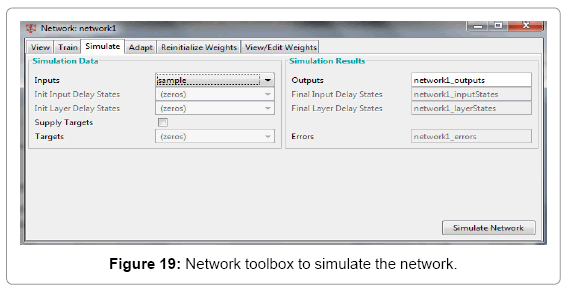
Figure 19: Network toolbox to simulate the network.
STEP 9: Click on the ‘output data’ in the Network/ data manager toolbox to view the output. The numerical value obtained gives the percentage of healthiness of the features of the given input image (Figure 20 and 21).
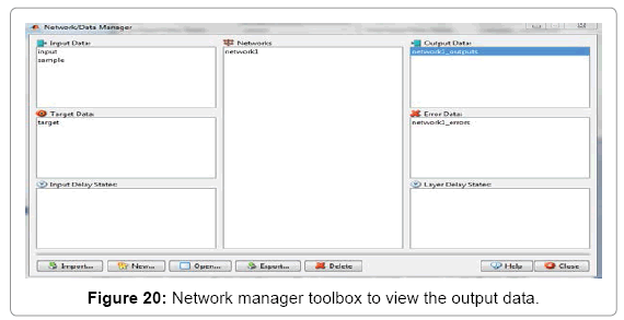
Figure 20: Network manager toolbox to view the output data.
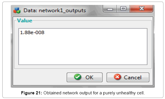
Figure 21: Obtained network output for a purely unhealthy cell.
By following the procedure mentioned above the pattern recognition output for the time series images is obtained by using feed forward backward propagation algorithm and the results are tabulated in Table 3 and Table 4, for the existing method, i.e., Segmentation using wavelet Otsu and feature extraction using GLCM and the proposed method i.e. Segmentation using hybrid wavelet Otsu curvelet algorithm and feature extraction using NSCT-GLCM technique. Hence the healthiness value of stem cell obtained from WOC+NSCT+GLCM+ANN is better than the WO+GLCM+ANN technique because of proficient segmentation and feature extraction (Table 3).
| Image | Healthiness value x100% |
|---|---|
| 0 hour | 1.88e-008 |
| 24 hour | 3.68e-006 |
| 48 hour | 0.046396 |
| 72 hour | 0.046888 |
| 96 hour | 0.40628 |
| 120 hour | 0.77153 |
| 144hour | 0.87431 |
| 168 hour | 0.9919 |
Table 3: Healthiness value x100% using WO+GLCM+ANN.
| Image | Healthiness value x100% |
|---|---|
| 0 hour | 0.0011131 |
| 24 hour | 0.0015252 |
| 48 hour | 0.14257 |
| 72 hour | 0.22169 |
| 96 hour | 0.56989 |
| 120 hour | 0.82368 |
| 144hour | 0.91431 |
| 168 hour | 1 |
Table 4: Healthiness value x100%using WOC+NSCT+GLCM+ANN.
In this paper, the healthy nature of the stem cells is evaluated. The time series images are affected by speckle noise hence wiener filter is used in pre-processing to remove the noise and to avoid the blurring that is caused due to anisotropic diffusion. The average PSNR value of anisotropic diffusion is 24%, by using wiener filter it has increased to 33%.Then the segmentation is performed using wavelet and Otsu segmentation techniques for which we get an average precision and recall value of 87.8% and 91% and the PSNR of 54%. In order to improve the precision recall and PSNR value and perform an efficient segmentation hybrid wavelet Otsu curvelet segmentation algorithm is performed. In which wavelet and curvelet have the property of multiresolution and multi-scaling then Otsu segmentation is performed using histogram analysis by which the complexity gets reduced and the precision, recall and PSNR get increased to 99.9%, 100% and 62% respectively. From the segmented image feature vectors are obtained by NSCT-GLCM feature extraction. Gray level co-occurrence matrix (GLCM) is an important method to extract the image texture features. However GLCM commonly extract the texture under single scale and single direction which does not provide the textural entities to its maximum extent. The set of feature vectors form finally the pattern matrix as the input to the artificial neural networks for their classification. This process is followed by the application of ANN for classification of feature vectors by the supervised learning process based on the feed forward network. Using neural network for pattern recognition, the network is trained by using the images of various healthy level images. Then using the trained network, the healthy nature of the test image is evaluated and the result is displayed in the form of percentage of healthiness of the given time series stem cell images.