Journal of Geology & Geophysics
Open Access
ISSN: 2381-8719
ISSN: 2381-8719
Review Article - (2017) Volume 6, Issue 3
Estimation of response profile in the soil layer from GPR synthetic data using forward modeling of radar data has been applied for reconstruction of 3 layers model without anomaly and 2 layers model with air-filled and water-filled cavity. For synthesizing the models, the reflection profiling and common mid-point (CMP) were used for the radar data in providing framework in order to link subsurface properties and GPR data. The result of the three layers model shows that response profile obtained is similar to lithology models using reflection profiling technique. Whereas, for the CMP the response profile gives oblique and hyperbolic patterns. For the two layers model, a diffraction response with wave travel time that longer in the side compared with the top of anomalous cavity is obtained using reflection profiling technique. Comparison to a GPR synthetic data model shows a good accuracy of the forward modeling.
Keywords: Ground penetrating radar; Forward modelling; Radar responses; Cavity; Anomaly
Ground-penetrating radar (GPR) surveys are high resolution electromagnetic technique, non-destructive and environmental friendly for shallow subsurface mapping [1]. The contrast in the electrical properties of the materials leading to reflections of electromagnetic waves is used in obtaining vital information about the subsurface structure [2]. In GPR target detection, the medium is generally considered as a non-magnetic medium. Therefore, the velocity of the electromagnetic wave is primarily determined by the relative permittivity of the medium [3-5]. Misinterpretations in the estimation or identification of subsurface material during field measurement are generally due to the presence multiple noises from materials which are not dominant/inhomogeneous. Inhomogeneity in the medium is as a result of variations in properties like the conductivity (σ), electric permittivity (εr) and magnetic permeability (μ) from point to point due to different composition of the media [3,5,6]. An important issue in forward modeling is the noise resulting from the collision of waves or wave readable by the response after alternating wave in the medium, and read with a uniform response. To overcome this problem, the modeling is conducted in such a way that the material that is not dominating is ignored to facilitate the anomalies response analysis.
The GPR modeling that is conducted in this study consists of soil layer models with forward modelings. Before measurement, the model is simulated with a purpose of estimating the responses from the target. In addition, the simulation could assist in estimating the physical parameters as well as the location of the material that is being measured or investigated. Whereas after measurement, the model’s simulation was made in order to facilitate the estimation of the reflection data process, in particular if model is estimated as soil layer with the raw data approach (drill data). In the literature, several works have been reported in respect to the application of Ground Penetrating Radar (GPR) method for subsurface mapping. A parallel 3-D staggered grid pseudo-spectral time domain method for ground penetrating radar wave simulation; 2-D permittivity and conductivity imaging by full waveform inversion of multioffset GPR data: a frequency-domain quasi-Newton approach; ground penetrating radar reflection attenuation tomography with an adaptive mesh [7-9].
Moreover, some studies relating to forward modeling of GPR have been investigated. These include: forward time domain GPR modeling of bridge decks for detecting deterioration multi-region finite difference time domain (FDTD) simulation for airborne radar; constructive inversion of vadose zone GPR observations, an approximate hybrid method for modeling of electromagnetic scattering from an underground target; effectiveness of 2-D and 2.5-D FDTD GPR modeling for bridge-deck deterioration evaluated by 3-D FDTD, pseudo-full-waveform inversion of borehole GPR data using stochastic tomography [10-15]. There are many analytical and numerical approaches taken by GPR researchers for forward modeling depending upon the application system. The study focused on forward modeling of GPR reflection data. The forward modeling conducted will be processed in a computational model of the soil layer is converted into a synthetic form. The forward modeling will be a combination of radar systems in two ways i.e. reflection pro-filling (monostatic or bistatik antenna) and the common mid-point (CMP) soundings. With the combination of the two radar systems, it is hoped can reduce the errors that arises in the estimation of response profile can be applied to minimize the misinterpretation due to the existence of ambiguity by multiple or noise.
The steps of making model
In this study, three hypothetical models were employed. For each of the models, the physical parameters used were represented as Tables. The model is created to fit the Earth’s subsurface using the reflex software. The procedure is shown in the following flowchart (Figure 1). The models are made using programs Demo-Version 4.2/93-98 refleks by K.J. Sandmeier Karlsruhe which has been equipped with GPRModel- Nondispersing [16].

Figure 1: Flow chart of GPR forward modeling.
The program is built on languages based computing with the Disk operation system (DOS) that can be run on the windows operating system. The program is based on the mathematical equations of electromagnetic waves propogating in a solid medium. An assumption made during the simulations was that a shallow soil with transmitter base frequency for both depth and size of target was adopted. A summary of the antennae geometries used for accurate modeling is represented in Table 1.
| Target depth Frequency Antenna (MHz) | Target Size (m) | Range Penetration (m) | Maximum Penetration (m) | Distance Antenna (m) |
|---|---|---|---|---|
| 25 | ≥ 1,0 | 5 to 30 | 35 to 60 | 4 |
| 50 | ≥ 0.5 | 5 to 20 | 20 to 30 | 2 |
| 100 | 0.1 to0.5 | 2 to 15 | 15 to 25 | 1 |
| 200 | 0.0 5to 0.5 | 1 to 10 | 5 to 15 | 0.6 |
| 400 | ≈ 0.05 | 1 to 5 | 3 to 10 | 0.6 |
| 1000 | Cm | 0.05 to 2 | 0.5 to 4 | 0 |
Table 1: Configuration of the frequency selection appropriate with the dimensions.
Base on the above configuration data, then modeling can continued with the making and determination of transmitter parameter of the simulation coordinate. Transmitter parameters are arranged with uniform layout so easier to recognize the differences profile is given. The transmitter parameters are:
• Travel time (t): 0.2357 ns
• Trace interval (x): 0.125 m
• Time-scaling: 1 ns
• Source: Plane wave
• Frequency: 100 MHz
The reflected wave is represented by a hyperbolic function (diffraction pattern). Mathematically, this can be explained using the expressions for reflection and refraction events in a two-layer model flat interface, with constant velocity when the offset is zero and the critical angle of incidence is small. Thus, satisfying equation (1):
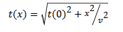
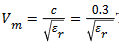
With t (0) in the zero-offset time, x the distance between the antennas and Ѵ is the velocity. Moreover, the velocity (Vm) of electromagnetic waves in a medium with low loss factor (P ≈ 0) is represented as
 Test models characteristics
Model A
Model A is a three-layered georadar model with different layer thickness. It is composed of air layer as topsoil. The second zone is clay sediments while wet sand layer represent the third layer. Geologically, model A could be simplified for an agricultural land use with depth less than 5 m. The geometry and Lithology of the model is shown in Figures 2a and 2b. Also, the parameters used for the simulation are presented in Table 2.

Figure 2: Schematic model for (a) estimates of geometry crosssection for a three layers (b) lithology model of a three layers.
| Media | εr | µr | σr |
|---|---|---|---|
| Air | 1 | 1 | 0.000001 |
| Clay | 10 | 1 | 0.000001 |
| Stone chip | 7 | 1 | 0.000001 |
Table 2: Physical parameters of the medium for model A.
Model B
This is a two-layered earth model with air as topsoil and limestone as second layer. The second layer contains an air-filled cavity. The geometries and lithology of the model B is shown in Figures 3a and 3b while the physical parameters used for the simulations are given in Tables 3

Figure 3: Schematic model for (a) estimates of geometri crosssection for a two layers and lithology models af a two layers with water-filled cavity.
| Media | εr | µr | σr |
|---|---|---|---|
| Air | 1 | 1 | 0.000001 |
| Limestone | 9 | 1 | 0.000001 |
| Water | 81 | 1 | 0.001 |
Table 3: Physical parameters of the medium for model B and C.
Model C.
This is another two-layered model but the second layer contains water-filled cavity. The geometry and lithology of the model is shown in Figures 4-6 while the physical parameters used for the simulations are given in Table 3.

Figure 4: Response profiles of a two layers model with (a) air-filled cavity (b) water-filled cavity by using wiggle plots.

Figure 5: Response profiles of a two layers model with (a) air-filled cavity (b) water- filled cavity.

Figure 6: The slices file of the snapshot for a two layers model with (a) air-filled cavity (b) water-filled cavity.
The results obtained for the three hypothetical models are presented as follows:
Three layered model
The three layers model is in the form of a sandy clay soils. These soils consist of humus (topsoil) weathering and a little dry sand on the top layers (layer 2) and the lower layer in the form of stone chips (layer 3). To view the response profile due to this layer, it is analyzed with wiggle plot using common mid-point (CMP) technique. The resulting raster is shown in Figures 7a and 7b. It is obvious that layer 2 (clay) is in time scale of less than 10 ns while layer 3 (stone chip) cannot be visualized and analyzed with the CMP method. This might be due to the presence of multiple reflections from layer 2.

Figure 7: Description of raster results for (a) raster of wiggle plot models of a three layers with common mid-point techniques (b) raster of the wiggle plot models of a three layers with reflection profiling techniques.
However, using equation 1 and 2, an approximate location of layers 3 can be obtained. The wave propagate in a medium of layer 2 corresponds to a velocity of 0.095 m/ns and distance of 2 m (where the surface of layer 3 is made in the material coordinate system ) with required time of 21 to 22 ns. If layer 3 is expected to occur at a depth of more than 20 ns, the layers 3 should be analyzed further by estimation of wave propagating velocity (need specific studies). While response profile which formed at a depth more than 50 ns is constitute reflected wave at hard basement.
Multiple that is shown Figure 8a is reading effect from two times or more reflections at same surface and always showing of the same amplitude for same surface. Multiple obtained from wave responses reflected by layer 3 then returns to surface of layer 2 and not directly to receiver, but still descent again to layer 3. Multiple reflections usually occurs in medium layers which mediates two surface of other layers. Multple can be identified with a uniform shape and almost fills the space inter-layers. Figure 8b shows the profile obtained using reflection profiling techniques and wiggle plot applied to determine the wave propagation velocities in the soil layers.

Figure 8: Description of raster results for (a) Raster of the pointmode plot models of a three layers with reflection profiling techniques and (b) the slices file of the snapshot of reflection-a and refraction-b waves.
The velocity of EM waves at layer 3 is 0.1134 m/ns using equation 2 for material with a permittivity of 7 F/m and on the assumption that wave propagation reaches the basement about 3 m from the surface of the layer 3. The required time is about 25 ns or more than 46 ns from soil surface of the layer 2. The results of the three layers model are shown in Figures 4a and 4b. They are obtained from the response profile similar with lithology models using reflection profiling. Whereas using common mid-point (CMP) soundings technique, the response profiles obtained are oblique and hyperbolic in shape. The effect of difference in the order of magnitude of the physical parameters of the material layer is shown with color of the amplitude response using the plot points-mode.
Figure 8a shows the radargram and at every time, there is an oscillation of a wave through the surface layer. At the surface of layer 2, the oscillation of the waves starts from 0 to positive order (the amplitude order of 285 to 585) and then up to the order more negative to the next layer. Based on equation 3, the amplitude of the radargram is influenced by the reflection coefficient. The reflection coefficient is dependent on the difference in wave propagation velocities in the two media (i.e., in this regards the propagation velocity is influenced by the permittivity of the material) as shown in Figure 8b. The radar responses that exhibit the pattern indicated by a is the reflected wave of layer 3. Whereas the pattern denoted by b is refracted wave which is passed by layer 3.
Two layered model with cavity
For the two layered model with cavity, the anomalies identified as shown in the response profiles in Figures 4a and 4b. For both models with the wiggle plot layer model of cavities filled water and air, the cavity is detected at depth of less than 30 ns beneath the surface. The response obtained is in the form of a hyperbola and it occurs after of wave reaches the upper end of the cavity.
In order to identify the difference in amplitude of cavity, the airfilled cavity gives an amplitude color range in order of positive values while the water-filled cavity gives amplitude color range in order of negative values.
Figures 5a and 5b obviously show responses in amplitude that distinguish both profiles. The shapes of the radar responses indicate that materials in the cavity are different. In the case air-filled, only the wave is partly transmitted whereas most of the wave is reflected to the cavity surface in the water-filled cavity. At the air cavity region, the reflected wave returned after reaching the basement of the cavity.
The anomalies responses of the transmitted wave in the air cavity and reflected wave in the water in the water-filled cavity due to absorption are shown in Figures 6a and 6b. This is as a result of difference in the permittivity of the materials with water having permittivity approximately 81 times than of air (i.e., εr=81 for water and εr=1 for air). As a result, EM wave passes easily in material with smaller permittivity compared with medium with higher value.
Forward modeling using Reflex program has been applied for the reconstruction of response profiles for air-filled and water-filled cavity in the soil layers. The response profile for a three layers model (without cavity anomalies) shows that similar lithology model is obtained using reflection profiling technique whereas the response profile obtained using CMP soundings are oblique and hyperbolic patterns in the soil layer. This confirms that the forward modeling method with a good understanding on the lithology of the investigated area is applicable for a good interpretation.
Moreover, the forwad modeling using the Reflex software of ground penetrating radar (GPR) can be used to minimize misinterpretation in the identification of subsurface material GPR data has been carried out. The misinterpretation may be caused by the multple and noise due to non-ideal condition of materials beneath the Earth surface. By forwad modeling, the multiple and noise can be reduced, that is by taking the dominant material as homogeneous or ideal condition. A profile/cross section model of the soil layer, the absorption properties of electromagnetic waves, is considered.
First of all we are thank to the Directorate General of Higher Education (DGHE) of Indonesia who has giving us scholarship. We thank to colleague at UHO-Kendari and Postgraduate student of Geophysics Programme, School of Physics, USM-Malaysia for their assistance.