Geophysical surveys are formed by data acquisition systems measuring different physical fields and signals, e.g., seismic, electromagnetic, gravity, and/or magnetic. These geophysical data acquisition systems use different sensors, and the data are collected on land, at the sea bottom, in a borehole, and from different moving platforms. Following Zhdanov [1], we can mathematically determine the sensitivity of geophysical survey as the ratio of the norm of perturbation of the observed data to the perturbation of the physical parameters of the medium under investigation. There exist a great variety of geophysical data acquisition systems, each of which has a specific sensitivity, determined by the physical nature of the measured data, the geometrical design of a system, and the configuration and type of the source of the recorded data. The sensitivity is usually limited to a specific “visible” part of the examined geological formation, located relatively close to the sensors.

It was demonstrated in Zhdanov [1] that, the size of this “visible” part of the examined formation can be determined based on an analysis of the integrated sensitivity of a survey, which allows the observer to evaluate a cumulative response of the observed data to the parameters of the examined target for a given data acquisition system. In a general case, the integrated sensitivity depends on many parameters, including the design of the geophysical survey, the properties of the measured geophysical field, and the configuration and type of the source of the observed data. Any given data acquisition system may have limited sensitivity (or limited resolution) to some sections of potential interest within the examined geological formation. The method of the calculation and optimization of the resolution of geophysical data was developed by Backus and Gilbert [2] and Parker [3] for linear geophysical problems. The Backus-Gilbert method is based on “narrowing” the data resolution function. In this paper we suggest a method of transforming the observed data in order to enhance their sensitivity to a particular zone of interest within a medium under investigation, and in order to increase the depth of investigation.

One way of solving this problem can be based on designing sources with specific radiation patterns, which would “steer” a generated field in the direction of an area of interest. This approach is implemented in the synthetic aperture method, which is widely used in radar, sonar, and seismic imaging [4-7]. A similar approach was recently discussed by Fan et al. [8], where the authors applied a synthetic aperture method to Marine Controlled-Source Electro-Magnetic (MCSEM) surveys. Their method used the interference of fields radiated by different sources to construct a virtual source with a specific radiation pattern, according to which the field is steered toward the target.

Another approach to achieving this goal is based on introducing data weights in order to increase the integrated sensitivity of the weighted data to a specific target area of subsurface formation. For example, it was demonstrated by Kaputerko et al. [9] that data weighting could dramatically affect the sensitivity distribution of a given survey. In the present paper, we demonstrate how the sensitivity of the Marine Controlled-Source Electro-Magnetic (MCSEM) survey could be “controlled” by selecting the appropriate data weights. Our approach is based on developing a general optimization method for the integrated sensitivity of a geophysical survey. This optimization can be reached by superimposing the recorded data with the corresponding weighting coefficients, which is physically equivalent to superimposing the sources and/or receivers. We introduce a method of designing the data weights in such a way that the new weighted data would have an integrated sensitivity with the desired (controlled) properties. This approach makes it possible to increase the resolution of a geophysical data with respect to potential subsurface targets. As an illustration, we apply this new technique to the sensitivity analysis of a typical marine Towed Streamer Electro-Magnetic (TSEM) survey.

Integrated Sensitivity

Consider a model, where the observed data d are related to the parameters of the examined medium m by a discrete operator equation:

d= A(m), (1)

where d=(d₁,d₂,d₃,…d_Nd) is a vector of the observed geophysical data, m= (m₁,m₂,m₃,…m_Nm) is a vector formed by the parameters of the examined medium in the model, and A is a forward modeling operator, which relates the model parameters to the observed data.

δd = Fδm (2)

where F is the sensitivity (Fréchet derivative) matrix of the forward modeling operator A. The technique of determining sensitivity matrix F for different geophysical fields is discussed in Zhdanov [1].

The integrated sensitivity of the data to parameter ämk is determined as the ratio of the norm of perturbation of the observed data, δd, to the corresponding perturbation of the parameters of the examined medium [1]:

(3)

The diagonal matrix with diagonal elements equal to is called an integrated sensitivity matrix:

(4)

Matrix S is formed by the norms of the columns of the Fréchet derivative matrix, F. Therefore, in order to compute the integrated sensitivity, one should determine the Fréchet derivative matrix, F. As discussed in Zhdanov [1], there are several approaches to solving this problem, based on direct sensitivity calculations using the finitedifference approach, and based on the reciprocity principles and its different variations. We refer the reader to the books by Zhdanov [1,10], where more details about calculation of the Fréchet derivative matrix for different geophysical fields can be found.

As an illustration, we consider a simple marine CSEM survey consisting of a horizontal electric bipole transmitter towed behind a boat and a set of towed horizontal electric dipole receivers (Figure 1). This marine data acquisition system has recently been developed [11]. The moving platform geometry enables the TSEM survey to be acquired over very large areas in both frontier and mature basins for higher production rates and relatively lower cost compared to conventional MCSEM surveys, characterized by arrays of fixed oceanbottom receivers and towed transmitters [12]. Figure 1 (top panel) shows, as an example, a typical towed marine streamer EM survey, where electric field data are generated by a 400 m long electric bipole transmitter moving in the x direction along a horizontal line at a depth of 10 m below the sea surface, and it is measured by an electric dipole receiver, towed at 2 km offset behind the transmitter at a depth of 100 m below the sea surface. The transmitter generates a frequency domain EM field with a frequency of 0.1 Hz and 0.75 Hz from the points, located every 100 m along the survey line, and the receiver measures the EX component of the electric field. The geoelectrical model consists of a seawater layer with a thickness of 1000 m, a resistivity of 0.33 Ohm-m, and a layer of conductive sea-bottom sediments with a resistivity of 1 Ohm-m. The bottom panel in figure 1 presents a vertical cross section of the integrated sensitivity distributions calculated using equation (4) for this towed TSEM survey. We can see that the integrated sensitivity decreases rapidly with the depth, indicating that the survey data are mostly sensitive to the upper layers of the sea-bottom formations. Note that, we show in figure 1 the sensitivity within the depth interval from 1500 m to 2500 m only, because the target area in the model is located within a depth interval from 1700 m to 1900 m, as shown in figure 2, top panel.

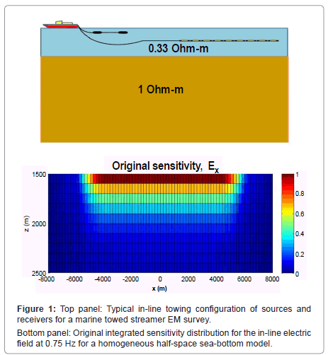
Figure 1: Top panel: Typical in-line towing configuration of sources and receivers for a marine towed streamer EM survey.
Bottom panel: Original integrated sensitivity distribution for the in-line electric field at 0.75 Hz for a homogeneous half-space sea-bottom model.

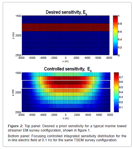
Figure 2: Top panel: Desired a priori sensitivity for a typical marine towed streamer EM survey configuration, shown in figure 1.
Bottom panel: Focusing controlled integrated sensitivity distribution for the in-line electric field at 0.1 Hz for the same TSEM survey configuration.

Definition of the focusing controlled sensitivity

The goal of this paper is to introduce the concept of focusing controlled sensitivity, which enables the sensitivity of a geophysical survey to be focused on a specific target area of a geologic formation. In order to reach this goal, we can consider a transformation of the original data acquisition system for a given survey into a new data acquisition system by applying a linear operator to the data recorded by the original survey:

d_c= W_cd, (5)

Where W_c is the rectangular matrix, describing the parameters of this transformation. The integrated sensitivity matrix of the new data acquisition system to the parameter δm is determined according to the following formula:

Applying the variational operator to both sides of equation (1), we obtain:

(6)

The goal is to create a data acquisition system with a controlled sensitivity to the target, located within a specific area of interest. For example, as we discussed above, in the case of the TSEM survey shown in figure 1, top panel, we assume that the target area is located within a depth interval of 1700 m to 1900 m (Figure 2, top panel). It is shown in figure 1, bottom panel, that, the original integrated sensitivity rapidly decreases with the depth. We will discuss here the method of designing the parameters of the linear transformation, W_c which would increase the sensitivity of the survey to the specific target area T.

In order to solve this problem, we select an a priori integrated sensitivity matrix, P, having maximum values within the desirable (target) area of the examined medium (e.g., within the layer of the sea-bottom formation located between the 1700 m and 1900 m depth, as shown in figure 2, top panel). The a priori preselected integrated sensitivity matrix P can be defined as a diagonal matrix [P_kk], where index k corresponds to the parameter of the medium. The diagonal components P_kk of matrix P are selected in such a way that they have large values, P_large for the parameter m_K corresponding to the target area T, and small values, P_small elsewhere:

P_kk = P_large , if m_K is within T; P_kk= P_small, if m_K is outside T.

In order to create a geophysical survey with a controlled sensitivity to the target located within a specific area of interest, we require that the parameters of the transformation W_c, satisfy the following condition:

diag(F*W_c*W_cF) » P² (8)

where we define the dimensions of all corresponding matrices as follows:

P=[N_m×N_m], F=[N_d×N_m], W_c=[N_w×N_d] (9)

We introduce the following notations for [N_d×N_d] matrix W_c*W_c

Q=W_c *W_c, Q= [N_d×N_d] (10)

We call matrix Q a kernel matrix of the corresponding data acquisition system and the linear transformation (5). Note that, the kernel matrix Q is a Hermitian matrix: Q=Q*.

The kernel matrix Q for a given a priori integrated sensitivity matrix, P, can be found by solving a minimization problem for a least squares difference between the a priori preselected and controlled sensitivities:

φ(Q)=Spur[(F*QF-P²)* (F*QF-P²)=min (11)

where symbol “Spur” denotes a trace of the corresponding matrix.

The minimization problem (11) is solved using the corresponding methods of the regularized inversion theory [1]. After matrix Q is determined, we can find the parameters of the linear transformation, W_c, (the controlled weights) by solving another minimization problem.

φ(Q)=|| [(Q-W_C *W_C)* (Q-W_C*W_C) ||_f=min (12)

Where ||…||_f denotes the Frobenius norm of the matrix.

The minimization problems (11) and (12) are solved using the Regularized Conjugate Gradient (RCG) method. Technical details of the RCG method can be found in Zhdanov [1].

Once the data weighting kernel matrix, Q is determined, we can then find the controlled data weighting matrix, W_c and appropriately weight the data. The modified data are then inverted using existing 3D inversion/imaging algorithms to produce the inverse model of geologic formation, for which the sensitivity to particular zones of interest has been enhanced.

Model study

I present a model study to demonstrate how we can use controlled sensitivities to focus on an a priori volume of interest in an earth model. In what follows, we consider, as an example, the same typical marine TSEM survey, discussed above (Figure 1, top panel). We will use three different a priori sensitivity models. The first one is described by a layer within the sea-bottom formations (Figure 2, top panel). This layer could represent a sequence of horizons, which may include a hydrocarbonbearing reservoir (the target of marine CSEM surveys). The second one is described by a finite 2D vertical cross section within the sea-bottom formations (Figure 3, top panel), which could represent a region containing a hydrocarbon-bearing reservoir. The third one is a model of homogeneous constant sensitivity extended from the sea bottom to infinity (Figure 4).

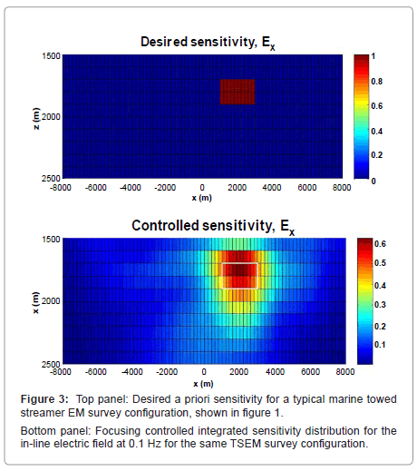
Figure 3: Top panel: Desired a priori sensitivity for a typical marine towed streamer EM survey configuration, shown in figure 1.
Bottom panel: Focusing controlled integrated sensitivity distribution for the in-line electric field at 0.1 Hz for the same TSEM survey configuration.

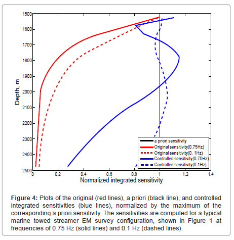
Figure 4: Plots of the original (red lines), a priori (black line), and controlled integrated sensitivities (blue lines), normalized by the maximum of the corresponding a priori sensitivity. The sensitivities are computed for a typical marine towed streamer EM survey configuration, shown in Figure 1 at frequencies of 0.75 Hz (solid lines) and 0.1 Hz (dashed lines).

The developed method has been applied to the synthetic TSEM survey, introduced above (see Figure 1, top panel). The sensitivity of the original TSEM survey rapidly decreases with the depth, as shown in figure 1, bottom panel. In the first example, we select an a priori sensitivity having maximum values within the given depth range of the sea-bottom formations; this preselected (desired) a priori sensitivity is shown in figure 2, top panel. As we discussed, we set the maximum values of the a priori sensitivity within the target area ranging from 1700 m to 1900 m depth, as shown in figure 2. We now apply the developed method to transform the original survey data into new data with the controlled integrated sensitivity, by solving a minimization equation (11) for a least squares difference between the preselected and controlled sensitivities. Figure 2, bottom panel, presents the distribution of the focusing controlled integrated sensitivity for the in-line electric field E_x at 0.1 Hz. This controlled sensitivity has its maximum values within the targeted interval from 1700 m to 1900 m, as it is required by the a priori sensitivity.

In the second example, we select the desired a priori sensitivity, having maximum values within a specific local target area, shown in figure 3, top panel. After application of the developed method, we have transformed the original TSEM survey data into new data with the controlled sensitivity focused on the predetermined target area, as shown in figure 3, bottom panel.

The results presented in these two examples raise the question, is it possible to increase the sensitivity of geophysical surveys up to any desirable depth? The laws of physics tell us that this should not be possible, because the sensitivity depth of any data acquisition system is limited by the natural decrease of the response with the depth of the target. It is obvious that, no mathematical manipulation can increase the survey sensitivity up to an arbitrary depth. There should exist some maximum possible sensitivity/depth curve for a given geophysical survey, determined by the corresponding physical properties of the corresponding geophysical data. In this situation, the method of controlled sensitivity should provide an estimate of this curve, which we call the Sensitivity Limit (SL) curve for a given geophysical survey.

The final example illustrates the principles of SL curve determination for the synthetic TSEM survey, introduced above (Figure 1, top panel). In this case, we assume that, the desired survey would have homogeneous constant a priori sensitivity extended from the sea bottom to infinity, as shown by the vertical black line in figure 4. The plots of the original integrated sensitivities normalized by their maximum values are shown by the red lines. The sensitivities are computed for a typical TSEM survey configuration, presented in figure 1, at frequencies of 0.75 Hz (solid line) and 0.1 Hz (dashed line). We now search for the survey with the optimal controlled sensitivity, which would best approximate the homogeneous constant a priori sensitivity. The blue lines in figure 4 show the corresponding controlled integrated sensitivities at frequencies of 0.75 Hz (solid line) and 0.1 Hz (dashed line), respectively. We may consider these controlled sensitivities as the corresponding SL curves for a given marine TSEM survey. One can see that the SL curve for the higher frequency (0.75 Hz) decays faster than the corresponding SL curve for the lower frequency (0.1 Hz), which corresponds well to the appropriate skin depth of the EM field. Thus, the concept of the sensitivity limit curves provides the possibility of appraising different possible survey configurations in order to select the optimal geophysical survey with the maximum sensitivity range.

I have introduced the concept of controlled sensitivity, which enables the sensitivity of geophysical surveys to be focused on a specific volume of interest where a potential target may be located. We have also developed a numerical method for constructing a synthetic survey with the desired sensitivity to the target. The method is based on the weighting and superposition of the recorded data in such a way that the new weighted data would have an integrated sensitivity with the desired (controlled) properties. This method does not require any modifications in the physical design of the given geophysical survey. The effect of focusing controlled sensitivity can be achieved by algebraic transformation of the conventional recorded data. I have illustrated the method with the example of the marine towed streamer EM survey data. However, the method can be applied to any geophysical survey, including seismic, electromagnetic, and potential field data. The developed technique can be used for producing images and inverse models of geologic formations with the enhanced sensitivity to particular zones of interest. More research is needed to study this approach for different geophysical surveys. This will be a subject of future papers.

I wish to acknowledge the support of the University of Utah Consortium for Electromagnetic Modeling and Inversion (CEMI) and TechnoImaging. I also thank Alex Gribenko and DaeUng Yoon for their assistance with the numerical model study.