Journal of Geology & Geophysics
Open Access

Evaluation and Assessments of Borehole Paleothermometry Methods for Inferring Past Climate Change

Wang Chen^{* *}Correspondence: Wang Chen, School of Sciences, Chang'an University, Xi'an, People's Republic of China, Email:

Author info »

Introduction

The recognition that past climate changes affects the subsurface temperature field dates back to Lane, et al. [1]. Since the work of Lachenbruch, et al. [2,3], there has been a significant number of works on the inference of a past Ground Surface Temperature History (GSTH) from borehole temperature-depth (T-z) measurements. Owing to the lack of accurate data, model parameterization and optimization (regularization) are required for a unique and stable solution for such an ill-posed numerical problem. A consequence is that the estimated GSTH depends on the inverse method used. The aim of this work is to examine the applicability and exactness of different inverse methods for different synthesis example data sets, and stability when adding random noise of different noise levels.

The application of modern geophysical inverse theories to the reconstruction of a GSTH from borehole T-z data began with the work of Vasseur, et al. [4], who used the Backus et al. [5], formalism. This formalism was also adopted by Clow, et al. [6]. However, two types of inverse methods have emerged as the most popular among researchers. One type is based on the method of least squares, specifically the nonlinear least squares inverse theory of Tarantola, et al. [7-10] and (e.g., Nielsen, et al. [11]; Shen, et al. [12,13]; Cermak et al. [14]; Lewis, et al. [15]; Safanda, et al. [16]; Sebagenzi, et al.[17]; Wang, et al. [18-20]; Shen, et al. [21]; Huang, et al. [22]; Pollack, et al. [23]; Rath, et al. [24]). Similar in principle is the control theory applied by MacAyeal, et al. [25], and Kakuta, et al. [26]. The other type of inversion method is based on the technique of singular value decomposition, or SVD [27,28], for solving systems of linear equations (e.g., Beltrami, et al. [29-31]; Mareschal, et al. [32,33]; Clauser, et al. [34,35]; Harris, et al. [36]). The readers are referred to Shen, et al. [12,13] and Mareschal, et al. [32], for descriptions of the FSI and SVD methods, respectively. We shall briefly describe the formulations of two new methods: MFS and Tikhonov methods. Both MFS and Tikhonov methods like SVD deal with a linear system after parameterization and use Tikhonov regularization and Generalized Cross Validation (GCV) for regularization parameter selection.

Three earlier comparative studies (Beck et al. [37]; Shen et al. [38,39]) confirm the wide range over which inverse results may vary. Because of different effectiveness of MFS and Tikhonov methods compared with others in inferring the Ground Surface Temperature History (GSTH) from borehole temperature data, several synthetic sets were prepared for comparison of four inversion methods: FSI, MFS, SVD and Tikhonov. In this study we seek and understanding of variability of different methods for different kinds of GSTHs, by means of simple synthetic experiments in the presence of different levels of noise. The ground temperature-depth profile data sets were synthetically generated by four forms of GSTHs and have been randomly perturbed by noise with different noise levels.

Materials and Methods

Inversion methods

All of these inverse methods based on the one-dimensional heat conduction theory. Shen’s functional space inversion method (Shen, et al. [12,13]) employ the least squares inverse theory of Tarantola, et al. [7,8]. Beltrami and Mareschal’s SVD method use the singular value decomposition for parameter estimation. Tikhonov method uses the Tikhonov regularization method to deal with the unstable linear system for parameter estimation. Fundamental solution method use fundamental solution function to express approximated GSTH and solve ill-posed linear system for the unknown parameter.

A large part of the discrepancies in the inverse results can therefore be attributed to the different regularizations imposed on the different mathematical theory basis in order to smooth and uniquely determine the inverse solution; such regularizations are necessary because the inverse problem is ill-posed. For example, Singular Value Decomposition method constrains the solution by eliminating the small singular values and their associated eigenfunction from consideration whereas Functional Space Inversion method constrains the solution by imposing various autocovariance functions on the GSTH. Fundamental solution method and Tikhonov method both utilize Tikhonov regularization technique imposed on different mathematical linear system in order to diminish their ill-posedness especially the instability. Another source of the discrepancies is, of course, the different mathematical basis, which means the different parameterization schemes used. For example, SVD and Tikhonov method constrain the GSTH to several step changes (see below) while the rest allow the GSTH to be a rather smooth function of time. Since detailed descriptions of FSI and SVD methods are readily available elsewhere (Shen, et al. [12]; Mareschal, et al. [32]), we shall describe briefly only the remaining two methods.

Let the conductive thermal regime be defined over the time interval [t₀, t_max] and the depth interval [z₀, z_max]. Then the temperature field θ(z,t) may be written as (Jaeger, et al. [40]),

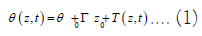
Here z is depth (positive downwards, in m), and t is time (yr), θ₀ is the pre-observational mean ground surface temperature or the steady state ground surface temperature (℃), and the linear part θ₀+Γ₀z denotes the initial steady temperature depth profile (℃). T(z, t) is the transient component (℃) due to surface disturbance.

The method of Tikhonov is similar to that of SVD method (Mareschal, et al. [32]). This method assumes a homogeneous, isotropic, source-free half space, the transient temperature perturbation is solution of the diffusion equation (Jaeger, et al. [40]),

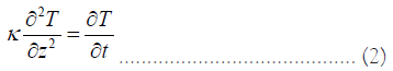
Here κ is the thermal diffusivity of the rock (m²∙s^-1). The ground surface temperature is represented by a series of temperature steps T_j^G at times t_j before present (t=0), the transient term becomes

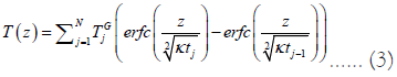
This lead to a set of linear algebraic equations which is ill-posed and need to be regularized. The principle difference between the Tikhonov method and that of SVD is the regularization techniques constrained on the solution, where the former employs the Tikhonov regularization (Tikhonov, et al. [41]) while the latter uses the singular value decomposition regularization.

The method of fundamental solution differs from the other methods principally in its forward solution and it employs the basis of the fundamental solution of heat equation (2). Unlike the SVD and Tikhonov methods, MFS method consider the temperature field in a bounded space with zero initial condition, upper boundary condition (i.e. the GSTH) and the lower zero boundary condition since the space interval is deep enough that surface temperature disturbance will not get to depth z_max. The fundamental solution of equation (2) is (Evans, et al. [42]),

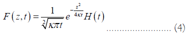
Here H(t)=1 if t ≥ 0 and H(t)=0 if t<0. Take some source points (x_j *, t_j *), j=1, 2 …, M and a positive real number τ that τ>max_j{t_j *}. All the source points are pair wise distinct on the spatial-time space boundary.

Following the idea of the method of fundamental solutions, we assume that an approximate solution to the inverse boundary value problem for equation (2) can be expressed by the following linear combination of basis functions

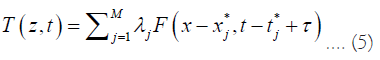
where λ_j are unknown coefficients to be determined. It is noted that the approximate solution has already satisfied heat equation (2) for t>0.

Take collocation points {(x_i, t_i), i=1, 2 …, M} on the initial time t=t₀, boundary z=zb, and end time t=t_max. By fitting the boundary condition with present time borehole T-z profile, we obtain a linear system.

Both Tikhonov and MFS methods are deal with ill-posed linear system with parameters to be determined. For the illposed problem of inversion of GSTH, the matrix resulting by a discretization will have a large condition number. In this study, we employ the Tikhonov regularization [41], and use the Generalized Cross Validation (GCV) method to determine the regularization parameter in the above two methods [43-45].

Synthetic experiments

In this paper we seek an understanding of variability yield from different methods by means of simple synthetic experiments which explore the way by which these four methods extract a climate signal in the presence of different levels of noise. In these experiments we treat five types of signals (Figure 1), a onestep signal, a single-ramp signal, a smooth single-ramp signal, a sinusoidal signal, and a mixed sinusoidal. Prior to 1000 years before present, all synthetics assume a uniform steady state surface temperature of 1℃ with steady ground temperature of ( ) 1 0.03 s U z = + z . Here z is depth underground (m). We assumed a typical rock or permafrost thermal diffusivity value of κ=1.2×10^-6m²s^-1. Specific expressions of four examples are provided as following.

Case 1 One-step type GST signal

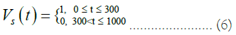
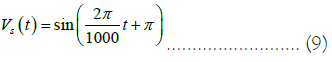
Here t is time before present (year), Vs(t) is GST changes with time (℃) and the notes are same in Case 2-4.

Case 2 Single-ramp type GST signal

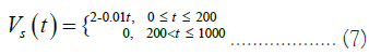
The single-ramp signal has amplitude of 2℃ and can be thought of as a simplified representation of a recent warming.

Case 3 Smooth single-ramp type GST signal

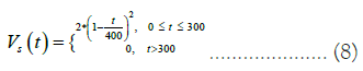
Compared with single-ramp signal, the smooth single-ramp signal has a more smoothed turning point, which simulate climate signal better.

Case 4 Sinusoidal type GST signal

The sinusoidal signal has a periodicity of 1000 years and a mean value of 0℃ over the thousand year interval of representation. It can be thought of as a simplified representation of a longtime naturally fluctuating climate.

Case 5 Mixed sinusoidal type GST signal

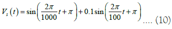
The mixed sinusoidal GST signal overlays a relatively high frequency simulated temperature cycle with periodicity of 100 years and mean value of 0℃. Here we set this case attempt to investigate resolve power of all methods.

The experiments are conducted as follows: Every synthetic signal is used in equation (3) to get the transient temperature-depth profile that perturbs the pre-existing steady state subsurface temperature. Random noise of varying amplitude is then added to the perturbed subsurface temperature, and the composite subsurface temperatures (steady state+transient+noise) are then inverted by all FSI, MFS, SVD, Tikhonov methods. Four levels of random noise have been considered: (a) 0℃, (b) 0.001℃, (c) 0.01℃, and (d) 0.1℃, respectively corresponding to idealized, very good, and fair field observations. The T-z profile is generated at 10 m intervals to a depth of 600 m, typical of many field T-z data sets.

The exact GSTH for these four examples and their noise-free temperature-depth (T-z) profile with steady state temperature for all synthetic examples are shown in Figure 1.

Figure 1: Temperature-depth (T-z) profiles for five kinds of GST variation with the steady ground temperature. The left panels are exact GST changes while the right panels are numerical T-z profiles (solid line) with steady state temperature (dotted line). Note: Steady temperature.

The reconstructions at each noise level we will later illustrate in Figures 2-5. Although simple in concept, the experiments probe both the signal dependence and the noise dependence of every inversion method.

Figure 2: Comparison of GSTHs for Case 1 inverted from four different methods of different noise levels with the true GST changes. The root mean square (RMS) errors are shown in the figure. Note: Tikhonov.

Figure 3: Comparison of GSTHs for Case 2 inverted from four different methods of different noise levels with the true GST variation; the synthetic data are derived by adding different levels σ of noise. Note: Tikhonov.

Figure 4: Comparison of GSTHs for Case 3 inverted from four different methods of different noise levels with the true GST variation; the synthetic data are derived by adding different levels σ of noise. Note: Tikhonov.

Figure 5: Comparison of GSTHs for Case 4 inverted from four different methods of different noise levels with the true GST variation; the synthetic data are derived by adding different levels σ of noise. Note: Tikhonov.

Results and Discussion

We now present the inverse results obtained by the four methods. For easy comparison, we group together the results for each data log. Thus Figures 2-5 give the results for synthetic example 1-4, respectively; in each figure the exact data inversion GST results variation is given at first, followed by noise level σ=0.001, 0.01, 0.1.

The FSI method copes with increasing level of noise by relaxing the significance attached to individual T-z and thermophysical property measurements (Shen, et al. [21]), resulting in a smoother, less detailed reconstruction with resolution restricted to more recent past. The FSI reconstructions estimate a steady-state slightly less or greater than that estimated by other methods. The main idea of the MFS is to approximate an unknown solution by a linear combination of fundamental solutions whose singularities are located outside the solution domain. So MFS is more suitable (Figures 2-6) to deal with the smooth synthetic example (like Case 4 and Case 5) than truncation function examples (like Cases 1-3). The selected regularization parameters of MFS at noise level of 0, 0.001, 0.01, and 0.1 are 5.6291e-014, 3.0238e- 016, 4.0482e-008, 1.3241e-007 respectively. The increasing of regularization parameter with noise level increase means the increasing ill-posedness and that the regularization plays more roles. At the core of SVD success in GSTH reconstruction is the availability of an adequate number of eigenfunctions to represent the GSTH, as noise is added to the subsurface temperatures, as increasing number of higher order eigenfunctions become dedicated in whole or in part to representing the noise, and must be discarded; thus fewer eigenfunctions are available for representing the GSTH. In this case, the SVD representation has retained only 9, 9, 7, 6 eigenfunctions for noise level σ=0, 0.001, 0.01, 0.1 respectively, corresponding least singular value are less than 0.005, 0.005, 0.05, 0.1. The difference between FSI, SVD, and Tikhonov methods in reconstructing the one-step signal, as shown in Figure 2, is small, and would suggest that either method can cope more or less equally with noise over a wide range of noise levels. When noise level is 0.001 and 0.01, which are the most measurement accuracy of borehole temperature, Tikhonov method get the most robust result than other methods. The regularization parameters for Tikhonov method are 5.0e-005, 0.0017, 0.0092, 0.0759 for different noise levels.

Figure 6: Comparison of GSTHs for Case 5 inverted from four different methods of different noise levels with the true GST variation; the synthetic data are derived by adding different levels σ of noise.Note: Exact GST, FSI,MFS, SVD, Tikhonov.

For Case 2, Tikhonov method is the most accurate except when noise level is of 0.1 and in all noise level situation this method get bester result of steady state temperature. FSI have the most power of suppressing noise disturbance but it get bad result when estimate the steady state surface temperature. The occasion near present time of FSI, SVD, Tikhonov methods are less than Case 1. Continuously change before 200 years seems better inverted than step change of Case 1 that all methods have smaller RMS errors than in Case 1. But the sharp corner still cannot be exactly approximate. The selected regularization parameters of MFS at noise level of 0, 0.001, 0.01, and 0.1 are 3.2929e-016, 3.2929e- 016, 6.2486e-015, 3.3249e-013 respectively. Retained numbers of eigenfunctions for SVD method are 14, 9, 7, 5, corresponding least singular value are less than 5e-6, 0.005, 0.05, 0.1. The regularization parameters for Tikhonov method are 0.0027, 0.0027, 0.0131, 0.0800 for different noise levels.

Same as Case 2, Tikhonov method is the most accurate except when noise level is of 0.1 and in all noise level situation this method get bester result of steady state temperature. And FSI have the most power of suppressing noise disturbance but it get bad result when estimate the steady state surface temperature. But the smooth corner can be perfectly approximate. The selected regularization parameters of MFS at noise level of 0, 0.001, 0.01, and 0.1 are 3.2929e-016, 8.8125e-015, 4.6182e-012, 3.7333e- 008 respectively. Retained numbers of eigenfunctions for SVD method are 11, 8, 7, 6, corresponding least singular value are less than 0.0005, 0.005, 0.05, 0.03. The regularization parameters for Tikhonov method are 1.0000e-004, 0.0035, 0.0189, 0.0767 for different noise levels.

For this sinusoidal case only MFS method gets the entirely robust result. Other methods only catch resent 200-300 years’ climate signal and have sharp vibration. The selected regularization parameters of MFS at noise level of 0, 0.001, 0.01, and 0.1 are 8.1658e-012, 8.1658e-012, 1.3611e-011, 1.1044e-012 respectively. Retained numbers of eigenfunctions for SVD method are 7, 7, 7, 7, corresponding least singular value are all less than 0.005. The regularization parameters for Tikhonov method are 0.0100, 0.0100, 0.0146, 0.0588 for different noise levels.

Same as sinusoidal case, mixed sinusoidal case has only MFS method gets the entirely robust general GST trend except the situation of high noise level of 0.1. FSI has better resolvent power of about recent 100 years’ high frequency signal than other methods. SVD and Tikhonov methods only catch resent 200- 300 years’ climate signal and have sharp vibration. The selected regularization parameters of MFS at noise level of 0, 0.001, 0.01, and 0.1 are 2.2691e-011, 3.9071e-12, 2.2691e-011, 2.6099e- 07 respectively. Retained numbers of eigenfunctions for SVD method are all 7, corresponding least singular value are all less than 0.005. The regularization parameters for Tikhonov method are 0.0175, 0.0177, 0.0220, 0.0572 for different noise levels.

Through general observations about the results, firstly, since all four methods are based on the same theory of 1-D heat conduction, we expect that they will give GSTHs that are similar in terms of their broadly trend. This is borne out by the results. Of course, the results differ significantly in terms of the timing of changes and in terms of the amplitude of changes, but this is to be expected because of the different parameterization schemes and regularizations imposed. Second, the presence of noise corrupts the inverse solution, as can be seen, for example. The portion of the GSTH that is most affected by data noise is the recent past (the last 100 years or so), where noise-induce oscillations (instability) are clearly visible (e.g., Figures 2, 5, and 6). This is a consequence of the nature of heat conduction, where the GSTH variations are damped exponentially and smoothed with depth (and time). The most recent GSTH variations is the part that is best resolved by the T-z profiles but it is also necessarily the part that is most susceptible to data noise. All four methods handle the effects of data noise by imposing regularizations on the solution, but apparently with varying degrees of success.

Figures 2-6 show that the FSI analysis achieves reasonably faithful GSTH reconstructions both 0.001℃ and 0.1℃ noise levels. In the most recent past the SVD and Tikhonov results exhibit greater oscillations than do the FSI results, and all exhibit greater oscillations than do MFS results. In the case of the sinusoidal and mixed sinusoidal signal, all FSI, SVD, Tikhonov inversions show virtually the same inability to resolve the early history of a diffusive process, yielding instead only the mean value of the temperature fluctuations in the interval of 600-1000 years before present. One easily sees the effect of increased noise: the loss of resolution in the middle of the 1000 year interval.

Conclusion

Our conclusion in this study is not that one of the four methods is superior to others in terms of GSTH reconstruction but all give good reconstructions in low-noise environments. The effectiveness of four methods becomes signal dependent. MFS method is more effective at recovering the sinusoidal signal and mixed sinusoidal signal. For other truncated function type of signal, Tikhonov method get the more exact results when adding noise is of levels 0.001 and 0.01. FSI deal with the noisiest data better than other methods for the truncated function signal but have higher or lower estimated steady state surface temperature. Also FSI method can reconstruct GST signal with higher frequency in recent years compared with other methods, but MFS can get more exact general trend of GST history.

We conclude with the following remark. Although the four inverse methods vary widely in their mathematical sophistication, all give reasonably good and similar results. The only exception are one-step type and mixed sinusoidal type, where the apparently diverse results may have been a consequence of the abnormally low GSTH signal relative to large noisy data in the synthesis data. Further investigation is warranted.

Acknowledgement

We thank Po-Yu Shen for his invaluable help and his original Fortran program code. The authors would like to thank the referee for valuable comments and suggestions which improved the presentation of this manuscript.

This research was supported by the National Natural Science Foundation of China (grant 41801029).

References

1. Lane AC. Geotherms of lake superior copper country. Geol Soc Am Bull. 1923;34(4):703-720.

   [Crossref] [Google Scholar]

2. Lachenbruch AH, Marshall BV. Changing climate: Geothermal evidence from permafrost in the Alaskan Arctic. Science. 1986;234(4777):689-696.

   [Crossref ] [Google Scholar] [PubMed]

3. Lachenbruch AH. Permafrost temperature and the changing climate. In Proceedings of the Fifth International Conference on Permafrost, Trondhelm, Norway. 1988;3:9-17.

   [Google Scholar]

4. Vasseur G, Bernard P, van de Meulebrouck J, Kast Y, Jolivet J. Holocene paleotemperatures deduced from geothermal measurements. Palaeogeogr Palaeoclimatol Palaeoecol. 1983;43(3-4):237-259.

   [Crossref ] [Google Scholar]

5. Backus GE, Gilbert JF. Numerical applications of a formalism for geophysical inverse problems. Geophys J Int. 1967;13(1):247-276.

   [Crossref] [Google Scholar]

6. Clow GD. The extent of temporal smearing in surface-temperature histories derived from borehole temperature measurements         . Glob Planet Change. 1992;6(2-4):81-86.

   [Crossref ] [Google Scholar]

7. Tarantola A, Valette B. Generalized nonlinear inverse problems solved using the least squares criterion. Rev Geophys. 1982;20(2):219-232.

   [Crossref] [Google Scholar]

8. Tarantola A, Valette B. Inverse problems=quest for information. J Geophys. 1982;50(1):159-170.

   [Google Scholar]

9. Tarantola A. Inverse Problem Theory. 1987;613.
10. Tarantola A. Theoretical background for the inversion of seismic waveforms, including elasticity and attenuation. Pure Appl Geophys. 1988;128(1):365-99.

    [Crossref ] [Google Scholar]

11. Nielsen SB, Beck AE. Heat flow density values and paleoclimate determined from stochastic inversion of four temperature-depth profiles from the Superior Province of the Canadian Shield. Tectonophysics. 1989;164(2-4):345-359.

    [Crossref ] [Google Scholar]

12. Shen PY, Beck AE. Least squares inversion of borehole temperature measurements in functional space. J Geophys Res. 1991;96(B12):19965-19979.

    [Crossref] [Google Scholar]

13. Shen PY, Beck AE. Paleoclimate change and heat flow density inferred from temperature data in the Superior Province of the Canadian sheild. Palaeogeogr Palaeoclimatol Palaeoecol. 1992;98(2-4):143-165.

    [Crossref ] [Google Scholar]

14. Cermak V, Bodri L, Šafanda J. Recent climate change recorded in the underground: Evidence from Cuba. Palaeogeogr Palaeoclimatol Palaeoecol. 1992;98(2-4):219-223.

    [Crossref ] [Google Scholar]

15. Lewis TJ, Wang K. Influence of terrain on bedrock temperatures. Glob Planet Change. 1992;6(2-4):87-100.

    [Crossref ] [Google Scholar]

16. Šafanda J, Kubík J. Evidence of ground surface temperature changes from two boreholes in the Bohemian Massif. Palaeogeogr Palaeoclimatol Palaeoecol. 1992;98(2-4):199-208.

    [Crossref] [Google Scholar]

17. Sebagenzi MN, Vasseur G, Louis P. Recent warming in southeastern Zaire (Central Africa) inferred from disturbed geothermal gradients. Palaeogeogr Palaeoclimatol Palaeoecol. 1992;98(2-4):209-217.

    [Crossref] [Google Scholar]

18. Wang K. Estimation of ground surface temperatures from borehole temperature data. J Geophys Res. 1992;97(B2):2095-2106.

    [Crossref] [Google Scholar]

19. Wang K, Lewis TJ. Geothermal evidence from Canada for a cold period before recent climatic warming. Science. 1992;256(5059):1003-1005.

    [Crossref ] [Google Scholar] [PubMed]

20. Wang K, Lewis TJ, Jessop AM. Climatic changes in central and eastern Canada inferred from deep borehole temperature data. Glob Planet Change. 1992;6(2-4):129-141.

    [Crossref] [Google Scholar]

21. Shen PY, Pollack HN, Huang S, Wang K. Effects of subsurface heterogeneity on the inference of climate change from borehole temperature data: Model studies and field examples from Canada. J Geophys Res. 1995;100(B4):6383-6396.

    [Crossref ] [Google Scholar]

22. Huang S, Shen PY, Pollack HN. Deriving century‐long trends of surface temperature change from borehole temperatures. Geophys Res Lett. 1996;23(3):257-260.

    [Crossref] [Google Scholar]

23. Pollack HN, Shen PY, Huang S. Inference of ground surface temperature history from subsurface temperature data: Interpreting ensembles of borehole logs. Pure Appl Geophys. 1996;147:537-550.

    [Crossref ] [Google Scholar]

24. Rath V, Mottaghy D. Smooth inversion for ground surface temperature histories: estimating the optimum regularization parameter by generalized cross-validation. Geophys J Int. 2007;171(3):1440-1448.

    [Crossref ] [Google Scholar]

25. MacAyeal DR, Firestone J, Waddington E. Paleothermometry by control methods. J Glaciol. 1991;37(127):326-338.

    [Crossref ] [Google Scholar]

26. Kakuta S. Surface-temperature history during the last 1000 years near Prudhoe Bay, Alaska: Applying control theory to the inversion of borehole temperature profiles. Glob Planet Change. 1992;6(2-4):225-244.

    [Crossref] [Google Scholar]

27. Lanczos C. Linear differential operators. 1961.
28. Jackson DD. Interpretation of inaccurate, insufficient and inconsistent data. Geophys J Int. 1972 ;28(2):97-109.

    [Crossref] [Google Scholar]

29. Beltrami H, Mareschal JC. Recent warming in eastern Canada inferred from geothermal measurements. Geophys Res Lett. 1991;18(4):605-608.

    [Crossref ] [Google Scholar]

30. Beltrami H, Mareschal JC. Ground temperature changes in eastern Canada: Borehole temperature evidence compared with proxy data. Terra Nova. 1993;5(1):21-28.

    [Crossref ] [Google Scholar]

31. Beltrami H, Mareschal JC. Resolution of ground temperature histories inverted from borehole temperature data. Glob Planet Change. 1995;11(1-2):57-70.

    [Crossref ] [Google Scholar]

32. Mareschal JC, Beltrami H. Evidence for recent warming from perturbed geothermal gradients: Examples from eastern Canada. Clim Dyn. 1992;6:135-43.

    [Crossref] [Google Scholar]

33. Mareschal JC, Vasseur G. Ground temperature history from two deep boreholes in central France. Palaeogeogr Palaeoclimatol Palaeoecol. 1992;98(2-4):185-192.

    [Crossref] [Google Scholar]

34. Clauser C, Huenges E. KTB thermal regime and heat transport mechanisms-current knowldege. Sci Drill. 1993;3:271-281.

    [Google Scholar]

35. Clauser C, Mareschal JC. Ground temperature history in central Europe from borehole temperature data. Geophys J Int. 1995;121(3):805-817.

    [Crossref ] [Google Scholar]

36. Harris RN, Chapman DS. Climate change on the Colorado Plateau of eastern Utah inferred from borehole temperatures. J Geophys Res. 1995;100(B4):6367-6381.

    [Crossref] [Google Scholar]

37. Beck AE, Shen PY, Beltrami H, Mareschal JC, Šafanda J, Sebagenzi MN, et al. A comparison of five different analyses in the interpretation of five borehole temperature data sets. Glob Planet change. 1992;6(2-4):101-112.

    [Crossref ] [Google Scholar]

38. Shen PY, Wang K, Beltrami H, Mareschal JC. A comparative study of inverse methods for estimating climatic history from borehole temperature data. Glob Planet Change. 1992;6(2-4):113-127.

    [Crossref] [Google Scholar]

39. Shen PY, Pollack HN, Huang S. Inference of ground surface temperature history from borehole temperature data: A comparison of two inverse methods. Glob Planet Change. 1996;14(1-2):49-57.

    [Crossref ] [Google Scholar]

40. Jaeger JC, Carslaw HS. Conduction of heat in solids. Oxford. 1959.
41. Tikhonov AN, Arsenin VY. Methods of solving ill-posed problems. Scr Ser Math. 1979.
42. Evans LC. Partial differential equations. 1988.
43. Craven P, Wahba G. Smoothing noisy data with spline functions: Estimating the correct degree of smoothing by the method of generalized cross-validation. Numer Math. 1978;31(4):377-403.

    [Crossref ] [Google Scholar]

44. Hanke M, Hansen PC. Regularization methods for large-scale problems. Surv Math Ind. 1993;3(4):253-315.

    [Google Scholar]

45. Wahba G. A survey of some smoothing problems and the method of generalized cross-valication for solving them. In Applications of Statistics. 1976;507-523.

    [Google Scholar]