Journal of Geology & Geophysics
Open Access
ISSN: 2381-8719
ISSN: 2381-8719
Research Article - (2013) Volume 2, Issue 2
The stress field along a plate margin is one of the basic tools for forecasting the magnitude of future earthquakes. Tectonic features like faulting, folding, fracturing and volcanoes are the results of stresses that build up along different fault lines across the world. Stress drop is a fundamental parameter of earthquakes. It is important to know how much portion of stress energy is released by an earthquake. Another important source parameter of earthquakes is repeat time, or the reoccurrence period of earthquakes. The reoccurrence period or repeat time of earthquakes is controlled by the rate of tectonic loading which is the long term slip rate, stress accumulation and stress drop. Earthquakes with long reoccurrence period have a higher average stress drop than those with short repeat time. The probability of reoccurrence of earthquakes is time dependent; which defines that some period is required to recharge stresses before they are released by a large earthquake. Time dependency of reoccurrence of a large earthquake is the base of earthquake forecasting. In this project earthquake repeat time and stress drop is determine for different fault types. Results of this study provide a method to estimate important parameters of active faults including static and dynamic stress drop, rupture length, width and earthquake magnitudes. These parameters can be used for future earthquake forecasting and prediction.
Keywords: Earthquake, Stress, Magnitude, Forecasting
Earth, from the crust to the centre of the core, is divided into a number of layers on the basis of mineral composition, heat flow, and seismic discontinuities. Tectonically the lithosphere and asthenosphere are very important because these two layers are responsible for stressesto build up in the Earth’s crust and release in the form of the earthquakes. The lithosphere of earth is broken into different parts; each of them is called a tectonic plate. These plates are floating over dense asthenosphere in a complex pattern with a velocity of 2-3 cm/year resulting tectonic earthquakes. About 80 percent of natural earthquakes are tectonic earthquakes which provide evidence for the release of strain energy. Figure 1 is showing global seismic activity for shallow earthquakes from 1976 to 2005.This figure indicates the distribution of focal mechanism solutions (FMS) along different plate margins, which in term gives the distribution of stresses along plate margins. The distribution of FMS provides information about the relative magnitudes of the principal stresses [1].
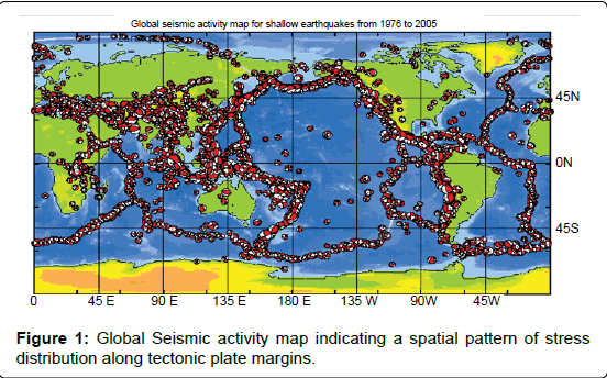
Figure 1: Global Seismic activity map indicating a spatial pattern of stress distribution along tectonic plate margins.
Tectonic features like faulting, folding, fracturing and volcanoes are results of stress fields. A stress field along a plate margin is one of the basic toolsfor forecasting the magnitude of future earthquakes. A most recent seismic activity in Tohoku, Japan (Magnitude 9.0 in 2011, According to USGS the 4th largest earthquake since 1900) was the result of long term stress built up along the pacific plate.The pacific plate is an oceanic plate subducting beneath the Eurasian Plate, forming a destructive plate margin. The friction between these two plates causes the stresses to build and release [2]. It is important to know how much portion of stress energy is released by an earthquake Figure 2. In the beginning of the 20th century, the earthquake sources werecharacterized on the basis of Richter Magnitude [3]. After the advancement in earthquake studies, parameters like seismic moments and stress drops are also introduced.
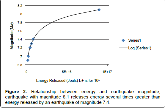
Figure 2: Relationship between energy and earthquake magnitude, earthquake with magnitude 8.1 releases energy several times greater than energy released by an earthquake of magnitude 7.4.
Earthquakes are the major source of reducing stress along a fault, which leads stress dropto be a fundamental parameter of earthquakes [4]. There exists a theoretical relationship between source parameters of earthquakes including the seismic moment, stress accumulation, stress drop, rupture length and fault displacement. Initial stress along a fault and stress drop gives information about seismic energy released during an earthquake [5]. Another important source parameter of earthquakes is repeat time, or the reoccurrence period of earthquakes. The reoccurrence period or repeat time of earthquakes is controlled by the rate of tectonic loading which is the long term slip rate, stress accumulation and stress drop. Earthquakes with long reoccurrence period havea higher average stress drop than those with short repeat time [6]. In the following section, relationships between all source perimeters of earthquakes are discussed in detail.
Tectonic earthquakes are related to active faulting in an area; therefore, parameters characterizing the source of an earthquake includes the rupture length “L” along a fault plane, the cross sectional area “A” of the fault , the mean slip on the fault “Smean”, the maximum surface displacement Dmax and the material property “µ”of the medium. These parameters are used to measure the stress drop “Δσ” after an earthquake by the following empirical scheme:
 (1)
(1)
Δσ is stress drop, SMean is mean slip, L is length of fault and µ is material property of medium while C is the shape factor and nearly equal to 1 for all fault classes [7].
The rupture length “L” can be obtained by using a scaling relationship [5].
 (2)
(2)
“Mo” is seismic moment can be determined by the following relation: Mo= µ A Smean
The stress drop along a fault line can also be obtained by calculating energy radiated by an earthquake. According to Richter [3], the energy radiated by an earthquake can be obtained by the following relation:
 (3)
(3)
Where Mw is Guttenberg and Richter unified magnitude. The relationship between seismic moment M0 and stress drop is given below:
 (4)
(4)
Here, µ is the rigidity of material for the crust is about 3*1011 dyne/ cm2
Example 1: By using the equation (3) and a catalog from The Geological Survey of Canada (available at http://www. earthquakescanada.nrcan.gc.ca/histor/top10-eng.php), energy released by the 8 largest earthquakes of Canadian is determined and given in Table 1.
| Date | Lat -N | Long-W | Magnitude | Energy(Joule) | Area Name |
| 12/23/1985 | 62.19 | 124.24 | 6.9 | 1.41*10^15 | NW Territories |
| 6/24/1970 | 51.77 | 130.76 | 7.4 | 7.94*10^15 | BC |
| 8/22/1949 | 53.62 | 133.27 | 8.1 | 8.91*10^16 | BC |
| 6/23/1946 | 49.76 | 125.34 | 7.3 | 5.6*10^15 | BC |
| 11/20/1933 | 73 | 70.75 | 7.3 | 5.6*10^15 | NW Territories |
| 11/18/1929 | 44.5 | 56.3 | 7.2 | 3.98*10^15 | Newfoundland |
| 5/26/1929 | 51.51 | 130.74 | 7 | 1.995*10^15 | BC |
| 12/6/1918 | 49.62 | 125.92 | 6.9 | 1.412*10^15 | BC |
Table 1: Energy released by the 8 largest earthquakes of Canada.
Equation 2 describes the rupture length in terms of the magnitude of an earthquake and stress drop. In case of very large earthquakes (Δσ, stress accumulated before Earthquake - stress released after Earthquake will be small) the mean slip (Smean) became linearly proportional to fault lengths, because in this case, the rapture affects the entire seismic zone and produces events of different lengths. There are two models to determine stress drop and mean slip, one is the W model which determines these parameters in terms of rupture width and the second is L model which defines stress drop and slip in terms of rupture length. The slip along a fault can be obtained by equation 5 [8].
 (5)
(5)
Where A is cross sectional area of the rupture which is related to rupture length and width by the following equation:
Results
 (6)
(6)
Where W is the rupturing width, and L is the rupture length. These perimeters, together with moment magnitude, are used to determine slip and stress drop after an earthquake. Empirical relations discussed in the above section are used to determine reoccurrence time of an earthquake and maximum magnitude potential along an active fault, discussed in following section.
Seismic sources are divided into two types, fault specific and areal sources. Earthquakes occur along the active faults, a fault which has shown activity in last 1.8 Million years is called an active fault [9]. After the careful observation of fault parameters and related earthquake source parameters, a general relation for earthquake magnitude and rupture length can be written in the following form [5].
M=f(L) or M=f (D) or M=f(L,D) (7)
Equation 7 is used to determine the relationship for maximum earthquake potential in the following way:
Ms=1.43 log(L)+4.36 (8) [10], and Ms=2log(L)+1.33log(Δσ)+1.66 (8) [9].
Earthquake events along different faults across the world are selected for current analysis given in Tables 2-4. Parameters in the earthquake data set includeearthquake source parameters (magnitude, date, location and seismic moment) and fault parameters (rupture length (L) Width (W) and slip. These parameters are applied in the mathematical relationships which are discussed in the above section to calculate energy radiated by earthquakes, stress drop and repeat time.
| Location | Epicenter | Date | Normal | Ms | Mo (10^26Dyn-cm) | L1 (Km) | L2 (Km) | W (Km) | A (Km2) | Smax | Savg |
| USA, CA | Eureka Valley | 5/17/1993 | N | 5.8 | 1.5 | 4.4 | 16.7 | 7 | 117 | 0.02 | - |
| New Zealand | Edgecombe | 3/2/1987 | N | 6.6 | 6.3 | 18 | 32 | 14 | 448 | 2.9 | 1.7 |
| Greece | Kalamata | 9/13/1986 | N | 5.8 | 0.89 | 15 | 15 | 14 | 210 | 0.18 | 0.15 |
| North Yemen | Dhamer | 12/13/1982 | N | 6 | 3.64 | 15 | 20 | 7 | 140 | 0.03 | - |
| Greece | Corinth | 2/24/1981 | N | 6.7 | 10 | 15 | 30 | 16 | 480 | 1.5 | - |
| Greece | Corinth | 2/25/1981 | N | 6.4 | 3.28 | 19 | - | 16 | 400 | 1.5 | 0.6 |
| Italy | South Apennines | 11/23/1980 | N | 6.9 | 26 | 38 | 60 | 15 | 900 | 1.15 | 0.64 |
| Greece | Thessaloniki | 6/20/1978 | N | 6.4 | 5.02 | `9.4 | 28 | 14 | 392 | 0.22 | 0.08 |
| Turkey | Gediz | 3/28/1970 | N | 7.1 | 67 | 41 | 63 | 17 | 1071 | 2.8 | 0.86 |
| Turkey | Alasehir Valley | 3/28/1969 | N | 6.5 | 13 | 32 | 30 | 11 | 330 | 0.82 | 0.54 |
| USA MT | Hebgen Lake | 8/18/1959 | N | 7.6 | 95 | 26.5 | 45 | 17 | 765 | 6.1 | 2.14 |
| USA, Nevada | Rainbow Mountain | 7/6/1954 | N | 6.3 | 2.4 | 18 | 11 | 14 | 252 | 0.21 | 0.25 |
| USA, Nevada | Stillwater | 8/24/1954 | N | 6.9 | 7.6 | 34 | 26 | 14 | 428 | 0.76 | 0.45 |
Table 2: Fault parameters, Normal Faults.
| Location | Fault name | Date | Reverse | Ms | Mo (10^26 Dyn-cm) | L1 (Km) | L2 (Km) | W (Km) | A (Km2) | Smax | Savg |
| Canada | Ungava | 12/25/1989 | R | 6.3 | 1.04 | 10 | 10 | 5 | 50 | 2 | 0.8 |
| Algeria | Chenoa | 10/29/1989 | R | 5.7 | 1.04 | 4 | 15 | 10 | 150 | 0.13 | - |
| Australia | Tenant Creek | 1/22/1988 | R | 6.3 | 2.8 | 10.2 | 13 | 9 | 117 | 1.3 | 0.63 |
| China | Wuqai | 8/23/1985 | R | 7.3 | 24.6 | 15 | 12 | 1.55 | - | ||
| USA, CA | Coalinga | 6/11/1983 | R | 5.4 | 0.15 | 3.3 | 8 | 6.5 | 52 | 0.64 | - |
| Algeria | El Asnan | 10/10/1980 | R | 7.3 | 50.8 | 31.2 | 55 | 15 | 825 | 6.5 | 1.54 |
| Iran | Tabas e Golshan | 9/16/1978 | R | 7.5 | 137 | 85 | 74 | 22 | 1628 | 3 | 1.5 |
| Australia | Caudex | 6/2/1979 | R | 6.1 | 1.67 | 15 | 16 | 6 | 96 | 1.5 | 0.5 |
| Turkey | Lice | 9/6/1975 | R | 6.7 | 7.4 | 26 | - | 13 | 234 | 0.63 | 0.5 |
| Iran | Karzin | 4/10/1972 | R | 6.9 | 15 | 20 | 34 | 20 | 680 | 0.1 | - |
| Japan | Senya | 8/31/1896 | R | 7.2 | 140 | 40 | - | 21 | 840 | 4.4 | 2.59 |
Table 3: Fault parameters, Reverse faults.
| Location | Fault Name | Date | Strike Slip | Ms | Seismic Moment (10^26 Dyn-cm) | L1 (Km) | L2 (Km) | W (Km) | A (Km2) | Smax (m) | Savg (m) |
| USA, CA | Landers | 6/28/1992 | RL | 7.6 | 114 | 71 | 62 | 12 | 744 | 6 | 2.95 |
| USSR | Armenia | 12/7/1988 | RL | 6.8 | 15.3 | 25 | 38 | 11 | 418 | 2 | - |
| USA, CA | San Francisco | 4/18/1906 | RL | 7.8 | 790 | 432 | 12 | - | 5184 | 6.1 | 3.3 |
| USA, CA | Imperial Valley | 5/19/1940 | RL | 7.2 | 27 | 60 | 45 | 11 | 660 | 5.9 | 1.5 |
| USA, CA | Kern County | 7/21/1952 | R-LL | 7.7 | 77 | 58 | - | 18 | 1080 | 4.35 | 2.1 |
| USA, CA | Park-field | 6/28/1966 | RL | 6.4 | 2.7 | 38.5 | 35 | 10 | 350 | 0.2 | - |
| USA, CA | Borrego Mountain | 4/9/1968 | RL | 6.8 | 10 | 31 | 40 | 10 | 400 | 0.38 | 0.18 |
| USA, CA | San Francisco | 2/9/1971 | RL-N | 6.5 | 10.4 | 16 | 17 | 14 | 238 | 2.5 | 1.5 |
| USA, CA | Oroville | 8/1/1975 | N-RL | 5.6 | 1.18 | 3.8 | 8 | 10 | 80 | 0.06 | - |
| USA, CA | Homestead | 3/15/1979 | RL | 5.6 | 0.241 | 3.9 | 6 | 4 | 24 | 0.1 | 0.05 |
| USA, CA | Green Vile | 1/24/1980 | RL | 5.9 | 0.6 | 6.2 | 11.5 | 12 | 138 | 0.03 | - |
| USA, CA | Coalinga | 6/11/1983 | R | 5.4 | 0.15 | 3.3 | 8 | 6.5 | 52 | 0.64 | - |
| USA, CA | Chalfont valley | 7/21/1986 | RL | 6.2 | 3.2 | 15.8 | 20 | 11 | 220 | 0.11 | - |
| USA, CA | Elmore Ranch | 11/24/1987 | LL | 6.2 | 2.6 | 10 | 30 | 12 | 360 | 0.2 | - |
| USA, CA | Superstition Hills | 11/24/1987 | RL | 6.6 | 9.2 | 27 | 30 | 11 | 330 | 0.92 | 0.54 |
| USA, CA | Landers | 6/28/1992 | RL | 7.6 | 114 | 71 | 62 | 12 | 744 | 6 | 2.95 |
| Taiwan | Yule Juisu | 11/24/1951 | LL-R | 7.4 | 46 | 43 | - | 17 | 731 | 2.1 | - |
Table 4: Fault parameters, Strike slip faults.
The seismic moment for given fault parameters can be determined by the following theoretical relation:
Mo=2µAD (9)
Where µ is shear modulus, A is cross sectional area and D is average slip along the fault [6].
Example 1: Seismic moment: The crustal earthquake of 1959 in Hebgan Lake, USA with a magnitude of 7.6 and an average slip of 2.14 meters and rupture area 765 Km.
Mo = 9822.6*1023dny.cm
Mo = 9.82*1026dyn.cm Or 9.82*1019N.m
Now in the following section where the data was obtained by Wells and Coppersmith publication: the reoccurrence or repeat time of earthquakes is determined. Before determining reoccurrence time, the stress drop is calculated by the following mathematical relationship [5].
The dynamic stress drop (Δσ2) is determined by using equation (8), while the static stress drop, also known as the theoretical stress drop, is calculated by using equation (1). The static stress drop (Δσ1) for the given data set can be determined by using C=1 and µ=3*1011 dyne/ cm2 in equation (1), while surface or subsurface rupture length and maximum displacement Smax or mean displacement Smean are obtained from Tables 2-4.
The data set obtained from Wells and Coppersmith is sorted on the basis of slip type and presented in Table 2-4. As data set contains three types of slips; therefore, it is possible to determine static and dynamic stress drops for reverse, strike slip and normal faults. The data set from Table 4 can be used to create a model for static and dynamic stress drop againstthe rupture length and width to observe the behavior of stress drop for different fault parameters. In the following section, two examples are solved for static and dynamic stress drop.
Static stress drop:
Equation 1 is given as: 
C=fault geometry and is approximately equal to 1 for all fault types. All other parameters are given in Table 3.
Example 2: Static stress drop: Park field earthquake of 1966 with magnitude 6.4, L = 38.5Km, W = 10Km Smax=0.2 m. Using this data set in equation (1) give following results
Δσ1=0.015*107*10-5bar=1.56bar
Dynamic stress drop
Equation for dynamic stress can be derived from equation (8) which is given as
Ms=2 log(L)+1.33 log(Δσ)+1.66
Δσ2=10[(Ms-2log(L)-1.66)/1.33] (10)
Δσ2=15.1 bar, similarly
Example 3: Static and dynamic stress drop: 1951 Earthquake of Taiwan with magnitude 7.4, L=43 Km, W=17 Km, and Smax=2.1 m.
Δσ1=14.7
Δσ=10[(Ms-2log(L)-1.66)/1.33]
Δσ2=72 bar
It can be observed from these two examples that dynamic stress drop is higher than the static stress drop. Similarly, for three slip types, stress drop is measured and results are shown in the following section:
Strike slip
Stress drop for an earthquake with a strike slip source is determined by using the data set from Table 4 and the results are given below Table 5.
| Ms | L1(Km) | W(Km) | Sigma1 | Sigma2 | Sigma2/Sigma1 |
| 7.6 | 71 | 12 | 25.352 | 48.119 | 1.898 |
| 6.8 | 25 | 11 | 24.000 | 57.876 | 2.411 |
| 7.8 | 432 | - | 4.236 | 4.502 | 1.063 |
| 7.2 | 60 | 11 | 29.500 | 31.010 | 1.051 |
| 7.7 | 58 | 18 | 22.500 | 77.550 | 3.447 |
| 6.4 | 38.5 | 10 | 1.558 | 15.127 | 9.707 |
| 6.8 | 31 | 10 | 3.677 | 41.881 | 11.389 |
| 6.5 | 16 | 14 | 46.875 | 67.358 | 1.437 |
| 5.6 | 3.8 | 10 | 4.737 | 123.183 | 26.005 |
| 5.6 | 3.9 | 4 | 7.692 | 118.464 | 15.400 |
| 5.9 | 6.2 | 12 | 1.452 | 99.175 | 68.321 |
| 5.4 | 3.3 | 6.5 | 58.182 | 107.723 | 1.851 |
| 6.2 | 15.8 | 11 | 2.089 | 40.836 | 19.552 |
| 6.2 | 10 | 12 | 6.000 | 81.241 | 13.540 |
| 6.6 | 27 | 11 | 10.222 | 36.464 | 3.567 |
| 7.6 | 71 | 12 | 25.352 | 48.119 | 1.898 |
| 7.4 | 43 | 17 | 14.651 | 72.351 | 4.938 |
Table 5: Stress drop measurements for different earthquakes with a strike slip nature (For details please see Table-1 after references).
Table 5 Stress drop measurements for different earthquakes with a strike slip nature (For details please see Table 1 after references).
Results for strike slip: A plot for dynamic and static stress drop is shown in Figure 3. There is a considerable difference between dynamic and static stress drop. It is also observed that dynamic stress drop is greater than static stress drop.
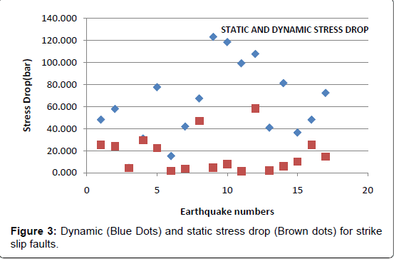
Figure 3: Dynamic (Blue Dots) and static stress drop (Brown dots) for strike slip faults.
The behavior of stress drop along the rupture width for a strike slip source is shown in Figure 4. From this figure, it can be observed that for smaller widths, the difference between dynamic and static stress drop is small (Figure 5). For large values of rupture width, the difference between dynamic and static stress drop decreases. Figure 4 also indicates that for shorter width (depth), which is brittle Earth, the stress drop by a small magnitude earthquake is higher, but as width (depth) increases, stress drop will also decrease, even for large magnitude earthquakes.
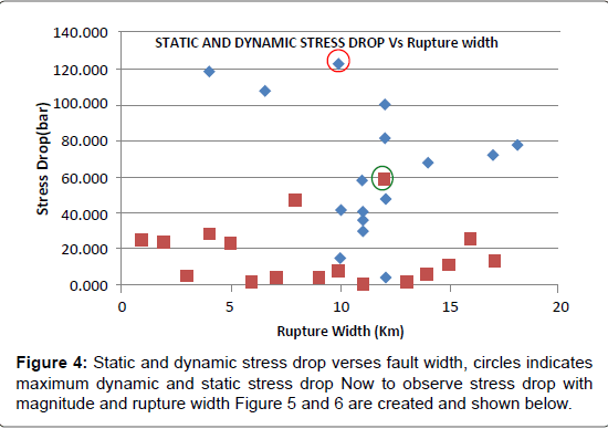
Figure 4: Dynamic (Blue Dots) and static stress drop (Brown dots) for strike slip faults.
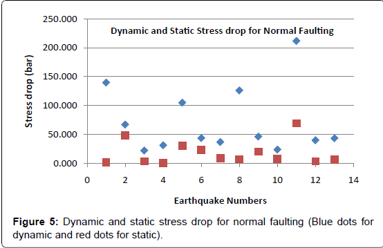
Figure 5: Dynamic and static stress drop for normal faulting (Blue dots for dynamic and red dots for static).
Reverse faults
In order to observe the behavior of stress drop with rupture parameters for reverse and normal sources (Figure 6), similar models are generated by using the data set from Tables 6 and 7.
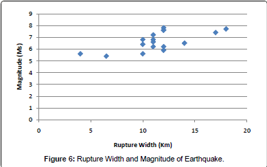
Figure 6: Rupture Width and Magnitude of Earthquake.
| Ms | L1(Km) | L2(Km) | W(Km) | A(Km2) | Smax(m) | Savg(m) | Sigma1 | Sigma2 | Sigma2/Sigma1 |
| 6.3 | 10 | 10 | 5 | 50 | 2 | 0.8 | 60.000 | 96.597 | 1.610 |
| 5.7 | 4 | 15 | 10 | 150 | 0.13 | - | 9.750 | 135.594 | 13.907 |
| 6.3 | 10.2 | 13 | 9 | 117 | 1.3 | 0.63 | 38.235 | 93.763 | 2.452 |
| 7.3 | 15 | 12 | - | 1.55 | - | 31.000 | 296.513 | 9.565 | |
| 5.4 | 3.3 | 8 | 6.5 | 52 | 0.64 | - | 58.182 | 107.723 | 1.851 |
| 7.3 | 31.2 | 55 | 15 | 825 | 6.5 | 1.54 | 62.500 | 98.572 | 1.577 |
| 7.5 | 85 | 74 | 22 | 1628 | 3 | 1.5 | 10.588 | 30.874 | 2.916 |
| 6.1 | 15 | 16 | 6 | 96 | 1.5 | 0.5 | 30.000 | 37.135 | 1.238 |
| 6.7 | 26 | - | 13 | 234 | 0.63 | 0.5 | 7.269 | 45.887 | 6.313 |
| 6.9 | 20 | 34 | 20 | 680 | 0.1 | - | 1.500 | 96.253 | 64.169 |
| 7.2 | 40 | - | 21 | 840 | 4.4 | 2.59 | 33.000 | 57.056 | 1.729 |
Table 6: Stress drop measurements for reverse type of faulting (For details please see Table-1 after references).
| Ms | Seismic Moment(10^26 Dyn-cm) | L1(Km) | L2(Km) | W(Km) | A(Km2) | Smax(m) | Savg(m) | Sigma1 | Sigma2 | Sigma2/Sigma1 |
| 5.8 | 1.5 | 4.4 | 16.7 | 7 | 117 | 0.02 | 1.364 | 139.696 | 102.444 | |
| 6.6 | 6.3 | 18 | 32 | 14 | 448 | 2.9 | 1.7 | 48.333 | 67.090 | 1.388 |
| 5.8 | 0.89 | 15 | 15 | 14 | 210 | 0.18 | 0.15 | 3.600 | 22.091 | 6.137 |
| 6 | 3.64 | 15 | 20 | 7 | 140 | 0.03 | - | 0.600 | 31.232 | 52.053 |
| 6.7 | 10 | 15 | 30 | 16 | 480 | 1.5 | - | 30.000 | 104.934 | 3.498 |
| 6.4 | 3.28 | 19 | - | 16 | 400 | 1.5 | 0.6 | 23.684 | 43.749 | 1.847 |
| 6.9 | 26 | 38 | 60 | 15 | 900 | 1.15 | 0.64 | 9.079 | 36.664 | 4.038 |
| 6.4 | 5.02 | 9.4 | 28 | 14 | 392 | 0.22 | 0.08 | 7.021 | 126.055 | 17.953 |
| 7.1 | 67 | 41 | 63 | 17 | 1071 | 2.8 | 0.86 | 20.488 | 46.237 | 2.257 |
| 6.5 | 13 | 32 | 30 | 11 | 330 | 0.82 | 0.54 | 7.688 | 23.753 | 3.090 |
| 7.6 | 95 | 26.5 | 45 | 17 | 765 | 6.1 | 2.14 | 69.057 | 211.810 | 3.067 |
| 6.3 | 2.4 | 18 | 11 | 14 | 252 | 0.21 | 0.25 | 3.500 | 39.911 | 11.403 |
| 6.9 | 7.6 | 34 | 26 | 14 | 428 | 0.76 | 0.45 | 6.706 | 43.338 | 6.463 |
Table 7: Stress drop for Normal faults. (For details please see Table-1 after references).
Results for reverse slip: It is observed that for reverse faults, the difference between static and dynamic stress is low, as compared to strike slip faults. In order to observe the behavior of stress drop for brittle (~up to 10Km) (Figure 7), and ductile (greater then 10Km) boundary, (Figures 8, 9) is created. This figure marks a boundary between brittle and ductile Earth at approximately 10Km where stress drop is highest (138 bar).
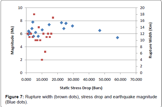
Figure 7: Rupture width (brown dots), stress drop and earthquake magnitude (Blue dots).
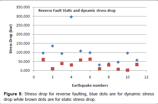
Figure 8: Stress drop for reverse faulting, blue dots are for dynamic stress drop while brown dots are for static stress drop.
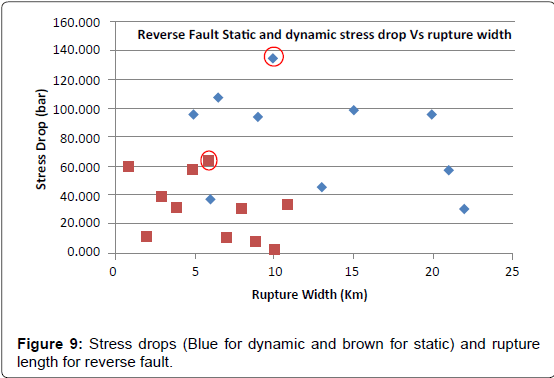
Figure 9: Stress drops (Blue for dynamic and brown for static) and rupture length for reverse fault.
Normal faults
Results for normal slip: From this section, it is concluded that earthquakes with reverse nature marks a well defined boundary between brittle and ductile zones. Energy released by earthquake or stress drop play an important role to determine reoccurrence time of earthquakes, discussed in following section.
The probability of reoccurrence of large earthquakes along an active fault is time dependent. The elastic rebound theory defines the reoccurrence of earthquakes on the basis of stress accumulation and stress drop. Time dependency of reoccurrence of a large earthquake is the base of earthquake forecasting. The probability of reoccurrence of earthquakes is time dependent; which defines that some period is required to recharge stresses before they are released by a large earthquake [11].
Repeat time of earthquakes along an active fault depends upon following parameters.
• Tectonic loading
• Stress accumulation
• Stress drop [6]
The data set for calculation of repeat timeincludes the seismic moment M or corresponding moment magnitude Mw, rupture length, width and magnitude (Ms). For this part of the project, data set for normal faults are selected for repeat time analysis. The following sources are used for data set preparation:
William L. Ellsworth, USGS [12],
Donald L. Wells and Kevin J. Coppersmith [13].
Calculations
Moment magnitude Mw
Moment magnitude can be calculated by the following equation
 (11)
(11)
Where Mo is the seismic moment discussed in the section above. The moment magnitude for a normal fault is measured by equation (11). It is then compared with the rupture length and repeat time. The results are shown in following section:
Example 5: For 1993, the earthquake of magnitue 5.8 with seismic moment 1.5*10^26dyn-cm, moment magnitude is given as
Mw = 6.7
Repeat time
Repeat time for an earthquake can be calculated by equation 12 [6]
 (12)
(12)
Where T is the repeat time in year, Smean is the mean slip along the fault and V is the slip rate which can vary for different tectonic zones.
Example 6: Reoccurrence time for an earthquake of magnitude 7.8 and mean slip of 3.3 meters along San Francisco fault can be determined in the following way:
An average slip rate along this fault is
T = 194.1 Years
Different faults have different slip rates, which depends upon their relative tectonic zone. For this part of project, slip rates for Normal faults (Table 7) are obtained from different sources and are shown in Table 8.
Now, by using data from Table 8 and the procedure from example 4, recurrence times are calculated for a normal slip and shown in Table 9. In the same way, repeat time can be determined for reverse and strike slip components can be calculated. From the table, it is observed that the slip rate plays an important role for the reoccurrence of larger earthquakes. In order to observe the relationship between rupture lengths, width and reoccurrence time of an earthquake, data can be shown in following way.
| Location | Fault | Slip Rate(mm/year) | Source |
| USA, CA | Eureka Valley | 3.5 | GSA |
| New Zealand | Edgecombe | 2.5 | GSN |
| Greece | Kalamata | 1 | NGA Data base |
| North Yemen | Dhamer | 0.36 | Web |
| Greece | Corinth | 2 | Kouvelas, 2005 |
| Greece | Corinth | 2 | Kouvelas, 2006 |
| Italy | South Apennines | 0.4 | Gori Et al 2012 |
| Greece | Thessaloniki | 0.1 | Zervopoulou et al 2007 |
| Turkey | Gediz | 4.3 | Buscher et al 2013 |
| Turkey | Alasehir Valley | 1 | Alasehir Valley |
| USA MT | Hebgen Lake | 2.5 | USGS |
| USA, Nevada | Rainbow Mountain | 0.5 | GSA |
| USA, Nevada | Stillwater | 0.3 | USGS |
Table 8: slip rates for earthquakes along normal fault.
| Location | Fault Name | Date | Ms | L | W | Savg | Slip Rate(mm/year) | Repeat Time (Year) |
| USA, CA | Eureka Valley | 5/17/1993 | 5.8 | 4.4 | 7 | 0.02 | 3.5 | 5.71 |
| New Zealand | Edgecombe | 3/2/1987 | 6.6 | 18 | 14 | 1.7 | 2.5 | 680.00 |
| Greece | Kalamata | 9/13/1986 | 5.8 | 15 | 14 | 0.15 | 1 | 150.00 |
| North Yemen | Dhamer | 12/13/1982 | 6 | 15 | 7 | 0.03 | 0.36 | 83.33 |
| Greece | Corinth | 2/24/1981 | 6.7 | 15 | 16 | 1.5 | 2 | 750.00 |
| Greece | Corinth | 2/25/1981 | 6.4 | 19 | 16 | 0.6 | 2 | 300.00 |
| Italy | South Apennines | 11/23/1980 | 6.9 | 38 | 15 | 0.64 | 0.4 | 1600.00 |
| Greece | Thessaloniki | 6/20/1978 | 6.4 | 9.4 | 14 | 0.08 | 0.1 | 800.00 |
| Turkey | Gediz | 3/28/1970 | 7.1 | 41 | 17 | 0.86 | 4.3 | 200.00 |
| Turkey | Alasehir Valley | 3/28/1969 | 6.5 | 32 | 11 | 0.54 | 1 | 540.00 |
| USA MT | Hebgen Lake | 8/18/1959 | 7.6 | 26.5 | 17 | 2.14 | 2.5 | 856.00 |
| USA, Nevada | Rainbow Mountain | 7/6/1954 | 6.3 | 18 | 14 | 0.25 | 0.5 | 500.00 |
| USA, Nevada | Stillwater | 8/24/1954 | 6.9 | 34 | 14 | 0.45 | 0.3 | 1500.00 |
Table 9: Repeat Time of Earthquakes.
It is observed that earthquakes with a higher magnitude have different ranges of reoccurrence time. While an earthquake with magnitude 6.4 has a repeat time of 800 years, another with a magnitude of 7.1 has a repeat time of 200 years (Figure 10). Also note that Earthquakes with magnitude 6.4 have a slip rate of 0.1mm/year, as one with a magnitude of 7.1 has a slip rate of 4.3 mm/year. This can be interpreted that the reoccurrence of large earthquakes is not only dependent on time for accumulation of stresses but also on the slip rate.
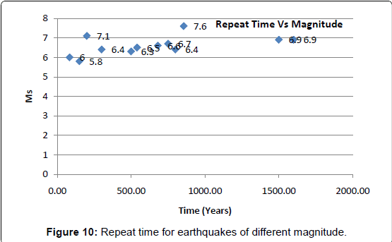
Figure 10: Repeat time for earthquakes of different magnitude.
Results from stress drop and reoccurrence time
From the first part of project, it is observed that the average stress drop along the reverse slip is higher as compared to normal and strike slip faults. Stress drop will increase with the rupture of width for a particular point, which is interpreted as the energy release along the brittle part of the Earth. Beyond that, the depth ductile nature appears and stress drop decreases with the increase of rupture width (Figure 11). Large earthquakes represent a large amount of release of strain energy and hence, larger stress drop. With the passage of time, energy starts to accumulate along active faults and releases in the form of strain energy after a particular period of time. This repeat time of energy release is not constant for a specific magnitude, but it also depends upon the slip rate along active faults. Table 10 and Figure 12 are the final results of this project.
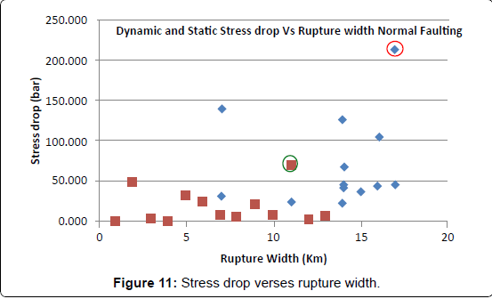
Figure 11: Stress drop verses rupture width.
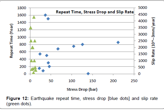
Figure 12: Earthquake repeat time, stress drop [blue dots] and slip rate (green dots).
| Location | Fault Name | Ms | Slip Rate(mm/year) | Repeat Time (Year) | Sigma2 | Energy Released (erg) |
| USA, CA | Eureka Valley | 5.8 | 3.5 | 139.696 | 3.16228E+20 | |
| New Zealand | Edgecombe | 6.6 | 2.5 | 680 | 67.09 | 5.01187E+21 |
| Greece | Kalamata | 5.8 | 1 | 150 | 22.091 | 3.16228E+20 |
| North Yemen | Dhamer | 6 | 0.36 | 83.33 | 31.232 | 6.30957E+20 |
| Greece | Corinth | 6.7 | 2 | 750 | 104.934 | 7.07946E+21 |
| Greece | Corinth | 6.4 | 2 | 300 | 43.749 | 2.51189E+21 |
| Italy | South Apennines | 6.9 | 0.4 | 1600 | 36.664 | 1.41254E+22 |
| Greece | Thessaloniki | 6.4 | 0.1 | 800 | 126.055 | 2.51189E+21 |
| Turkey | Gediz | 7.1 | 4.3 | 200 | 46.237 | 2.81838E+22 |
| Turkey | Alasehir Valley | 6.5 | 1 | 540 | 23.753 | 3.54813E+21 |
| USA MT | Hebgen Lake | 7.6 | 2.5 | 856 | 211.81 | 1.58489E+23 |
| USA, Nevada | Rainbow Mountain | 6.3 | 0.5 | 500 | 39.911 | 1.77828E+21 |
| USA, Nevada | Stillwater | 6.9 | 0.3 | 1500 | 43.338 | 1.41254E+22 |
Table10: Ms, Slip rate, repeat time, stress drop and energy release.
Faults with large repeat times have high probability of reoccurrence of large earthquakes in short period of time. While faults with smaller slip rates, results slow rate accumulation of energy and have high probability of reoccurrence after long period of time.