Journal of Chemical Engineering & Process Technology
Open Access

Dynamic Behavior of Mixing Tanks in Series

Duraid Fadhil Ahmed^{* *}Correspondence: Duraid Fadhil Ahmed, Department of Chemical Engineering, University of Tikrit, Tikrit, Iraq, Email:

Author info »

Abbreviations

C(t): Concentration (Kg/m³); D: Duration of the rectangular pulse (sec); G(s): Transfer function; h: Height of the rectangular pulse ( Kg/m³); KP: Steady-state gain (-); m(t): Force function; Q: Volumetric flow rate (m³/ hr); V: Volume of the mixing tank (m³); x(t): Response variable (Kg/m³); τ: Time constant of the mixing tank (sec)

Introduction

The process of mixing has a great importance in many processes. For example in chemical reactions the conversion of the reaction can be modified by the residence time distribution. The residence time distribution measures data associated with the bulk flow patterns or macro mixing in a process vessel. The mixing tanks are the most influential and therefore important units that a chemical engineer will encounter. To ensure the successful operation of mixing tanks it is necessary to understand their dynamic characteristics. A good understanding will ultimately enable effective control system design. There is a distinct difference between the steady state and dynamic behaviors of the mixing tanks especially when there is a recycle in the plant [1].

The performance of automatically controlled process plants depends on the dynamic interaction of all the components in the control loop. The dynamic characteristics of process components and of the overall plant indicated by frequency response data or by transient response data. From the control standpoint frequency response data are more useful. It is generally easier to compute the frequency response characteristics than the transient response characteristics since the frequency response is obtained directly from the transfer function of the process, while the transient response requires the taking of inverse Laplace transform.

The utility of mathematical models of chemical process is often limited by their complexity. Since exact analytical solutions to many important differential equations are unobtainable, the numerical calculations are often required for the comparison of theoretical prediction with observation. In the field of control system analysis, this difficulty has been circumvented by the employment of approximate models of physical system dynamics. Model parameters are estimated by sinusoidal or pulse testing techniques which require only the Fourier transform of the differential equation approximating the system.

In describing the experimental investigation of the dynamic behavior, the frequency response technique was chosen, as result obtained by this method is usually highly reproducible and is relatively easy to compare with prediction from theoretical models. This technique was applied in a number of dynamic studies of chemical process equipment. Including stirred tank reactor, heat exchanger and spray drier, turbulent flow system, bubble caps plates system and packed beds. This technique has been treated by Gangwall and Silveston, Al-Dawery, Wakao and Tanisho and Lokman [2-5]. Although this type problem has been treated in general terms by Lakshmann, Roetzel, Sharifi, Kahn and others [6-9].

The advantages of frequency response methods for the dynamic analysis of physical systems are well known. Some of the most fruitful techniques for process control and analysis are based on frequency response methods. One especially interesting use is the comparison of experimental frequency response data for a system with the response calculated for a postulated model, to obtain a quantitative estimate of the range of validity of the model in describing the system.

This paper presents a study of the dynamic characteristics of three mixing tanks in series by introducing rectangular pulse change in inlet concentration of the inlet stream and uses the frequency response analysis technique to evaluate the system model.

Materials and Methods

Mathematical model

A simplified representation of the three mixing tanks in series is shown in Figure 1. The mass balance for this process at any time is given by:

Mass flow in-Mass flow out=Mass accumulation in the tank

First tank

At steady state mass balance around the first tank at constant density:

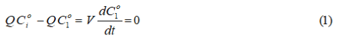
At unsteady state mass balance around the first tank at constant density:

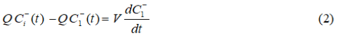
Subtracting the Equation (1) from Equation (2):

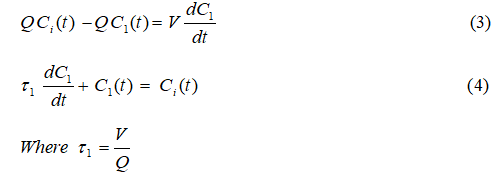
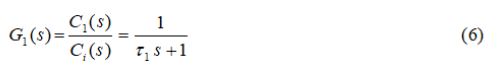
Assuming zero initial conditions, taking Laplace transformation of Equation (4)

The transfer function of the first tank is:

The same steps to derive the transfer function of the second and third tanks:

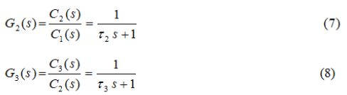
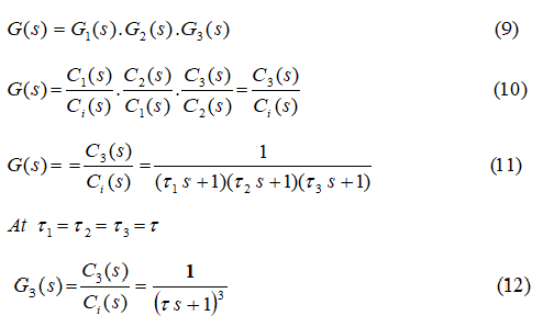
The overall transfer function of the three mixing tanks system is:

Frequency analysis

One of the most useful and practical methods for obtaining experimental dynamic data from many chemical engineering processes is pulse testing. It yields reasonably accurate frequencyresponse curves and requires only a fraction of the time that directs sine-wave testing takes.

An input pulse m(t) of fairly arbitrary shape is put into the process. This pulse starts and at the same value and is often just a square pulse (i.e., a step up at time zero and a step back to the original value at a later time t_m).

The input and output functions are then Fourier-transformed which then be used divided to give the system transfer function in the form of the frequency domain G(iω). The details of one procedure for accomplishing this Fourier transformation are discussed in the following sections and a little digital computer program. Alternative methods include the use of “Fast Fourier Transforms” which are available in most computing centers.

In theory only one pulse input is required to generate the entire frequency response curve. In practice several pulses are usually needed to establish the required size and duration of the input pulse. Consider a process with an input m(t) and an output x(t). By definition, the transformer function of the process is:

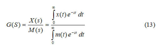
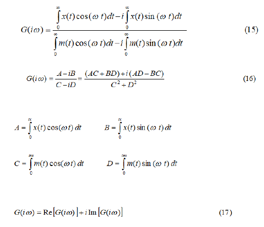
We now go into the frequency domain by substituting s=iω.

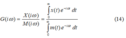
The numerator is the Fourier transformation of the time function x(t). The denominator is the Fourier transformation of the time function m(t). Therefore the frequency response of the system G(iω) can be calculated from the experimental pulse tests data x(t) and m(t).

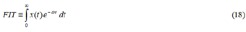
From Equation (14), we wish to evaluate the Fourier Integral Transform (FIT) of x(t).

We can break up the total interval (0 to t_x) into a number of unequal subintervals of length Δt_k. Then the FIT can be written, with no loss of rigor, as a sum of integrals:

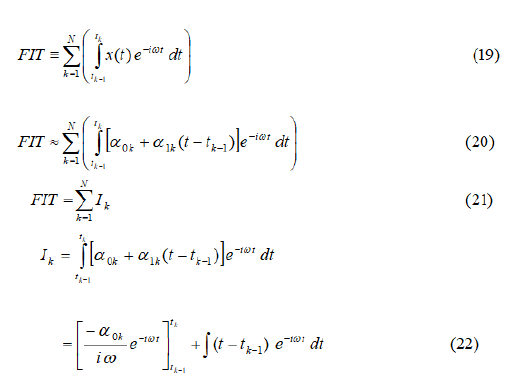
Each of the I_k integrals above can be evaluated analytically. Finally, the Fourier transformation of x(t) becomes:

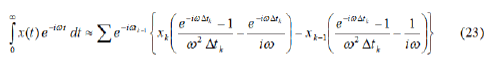
Equation (23) looks a little complicated but it is easily programmed on a digital computer. Appendix A gives a FORTRAN program that reads input and output time functions from a file, calculates the Fourier transformations of the input and of the output, divides the two to get the transfer function G(iω), and prints out log modulus and phase angle at different values of frequency. After obtaining the log modulus and phase angle, the Bode diagram can be plotted from which the system and transfer function can be obtained. This can represented the system model.

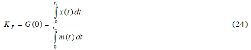
The steady state gain of the transfer function is G(0) or just the ratio of the areas under the input and output curves.

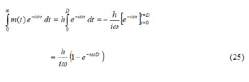
If the input pulse is a rectangular pulse of height h and duration D, its Fourier transformation is simply:

Description of the experimental equipment

A laboratory mixing tanks in series system is consisting of three mixing tanks, feed unit and measurement devices. The system is show in Figure 1. The essential part of this apparatus is three cylindrical mixing tanks of glass with a motor driven stirrer. The volume of this tank 0.66 liter with inlet and outlet streams and dip electrode which is fitted at the top of the tank to measure the conductivity of the solution in the tanks.

The pure water fed from 50 liter PVC tank to the head tank and the KCl solution at concentration 0.1 kg/m³ fed from 50 liter PVC tank to the head tank using two polypropylene centrifugal pump of capacity 25 lit/min against 1 m head of water. The rotameter having stainless steel float with range of flow (0.1-1 lit/ hr) of water at about 20°C each were employed for measuring the flow rate of the inlet streams.

Figure 1: Schematic diagram of three mixing tanks in series.

Experimental arrangement

The runs were carried out for the system, the equipment was first prepared as follows:

• Feeding tanks were filled with pure water and KCl solution.
• The pure water was then pumped to the mixing tank and then open three ways valve.
• Adjust the pure water to 0.4 lit/min by adjusting the valve to give a nominal reading on the rotameter and wait for steady state.
• The salt solution was then pumped to the mixing tank and changes the three ways valve from the pure water to the KCl solution and record the conductivity of the solution in the tanks.
• After 60 sec changing the three ways valve from the salt solution to the pure water and record the conductivity until reach to steady state.
• Repeat the steps 3, 4 and 5 for different flow rates at 0.5 and 0.6 lit/min and different duration of the pulse at 80 and 100 seconds.

Results and Discussion

The dynamic response of the three mixing tanks by rectangular pulse change in inlet concentration for different flow rates and different pulse duration are shown in Figures 2-7. This behavior can be approximated by a third order system with a time constant is equal from 66 second at 0.6 lit/min to 99 seconds at 0.4 lit/min. The response of the first tank is faster than second and third tanks because the first tank has one time constant while the second tank has two time constants and the third tank has three time constants. The response of the tanks at high flow rate is faster than the response at low flow rate because the time constant increase if the flow rate decrease.

The frequency domain modeling is the facility with which analytical frequency solutions can be obtained as compared with time solutions. However, the analytical inversion of the frequency solution to find the time solution is formidable. The lumped parameter model there is no change the form of the frequency solution as the values of the parameters change. The region of interest over which it is desired to fit a mathematical model is quite often conveniently expressed in the frequency domain.

Equations for the dynamic characteristics of a simple distributed system have been derived. The frequency response characteristics have been computed and it has been shown that distributed periodic forcing leads to resonance in magnitude ratio and phase lag angle. The Figures 8-13 show the frequency response characteristics of the three mixing tanks plotted on Bode diagram. The phase lag decrease from zero to (-90) with increasing frequency for first tank, (0 to -180) for second tank and (0 to -270) for third tank while log modulus decrease from zero to (-20) with increasing frequency for first tank, (0 to -40) for second tank and (0 to -60) for third tank. On the other hand the low flow rate computed curve lies higher than high flow rate. Part of this difference is due to the different time constant of the system at different flow rate.

The many problems it is much simpler and computationally advantageous to evaluate the model in the frequency domain. Another distinct advantage of frequency domain regression is that frequency domain specifications and restrictions can be easily incorporated. Frequency domain model evaluation allows one to take this into consideration; this may involve the elimination of a high or low frequency range or the rejection of a band of frequencies that perhaps contains noise or a spurious frequency component.

Figure 2: Experimental response of the first tank at pulse duration of 60 second for different inlet flow rate.

Figure 3: Experimental response of the first tank at flow rate of 0.4 lit/min for different pulse duration.

Figure 4: Experimental response of the second tank at pulse duration of 60 second for different inlet flow rate.

Figure 5: Experimental response of the second tank at flow rate of 0.6 lit/min for different pulse duration.

Figure 6: Experimental response of the third tank at pulse duration of 60 second for different inlet flow rate.

Figure 7: Experimental response of the third tank at flow rate of 0.6 lit/min for different pulse duration.

Figure 8: Bode plot of the first tank (log modulus) at pulse duration of 60 second for different inlet flow rate.

Figure 9: Bode plot of the first tank (phase angle) at pulse duration of 60 second for different inlet flow rate.

Figure 10: Bode plot of the second tank (log modulus) at pulse duration of 60 second for different inlet flow rate.

Figure 11: Bode plot of the second tank (phase angle) at pulse duration of 60 second for different inlet flow rate.

Figure 12: Bode plot of the third tank (log modulus) at pulse duration of 60 second for different inlet flow rate.

Figure 13: Bode plot of the third tank (phase angle) at pulse duration of 60 second for different inlet flow rate.

Conclusion

We conclude from the results the following points:

• The dynamic behavior of three mixing tanks in series can be approximated by a third order system and a closed fit between the theoretical model of the system and the model by using frequency response analysis.
• The response of the first tank to the rectangular pulse in inlet concentration is faster than second and third tank.
• The response of the tanks at high flow rate is faster than the response at low flow rate because the time constant increase if the flow rate decrease.
• The low flow rate computed curve in Bode diagram lies higher than high flow rate because of this behavior is due to the different in time constant of the system at different flow rate.

References

1. Amir AM, Mohmoud RM, Shahrokhi M. Analysis of control structure for recycled reaction/separation process with first order reaction. Pet Coal. 2006;48(1):48-60.

   [Google Scholar]

2. Gray RI, Prados JW. The dynamics of a packed gas absorber by frequency response analysis. AIChE J. 1963;9(2):211-216.

   [Crossref] [Google Scholar]

3. Al-Dawery SKH. neutralization process control based on pH and pION measurements. PhD’s Thesis, University of Nottingham. 1991.
4. Wakao N, Tanisho S. Chromatographic measurements of particle-Gas mass transfer coefficients at low Reynolds numbers in packed beds. Chem Eng Sci. 1974;29(9):1991-1994.

   [Crossref] [Google Scholar]

5. Abdulkareem LA. Modeling and control of a pressure-flow system based on advanced control techniques. Master’s Thesis, University of Baghdad. 2004.
6. Lakshmanan CC, Potter OE. Dynamic simulation of a countercurrent heat exchanger modelling-start-up and frequency response. Int Commun Heat Mass Transf. 1994;21(3):421-434.

   [Crossref] [Google Scholar]

7. Roetzel W, Xuan Y. Transient response of parallel and counterflow heat exchangers. ASME J Heat Transfer. 1992;114(2):510-511.

   [Crossref] [Google Scholar]

8. Sharifi F, Narandji MG, Mehravaran K. Dynamic simulation of plate heat exchangers. Int Commun Heat Mass Transf. 1995;22(2):213-225.

   [Crossref] [Google Scholar]

9. Khan AR, Baker NS, Wardle AP. The dynamic characteristics of a countercurrent plate heat exchanger. Int Commun Heat Mass Transf. 1988;31(6):1269-1278.

   [Crossref] [Google Scholar]