Journal of Medical Diagnostic Methods
Open Access
ISSN: 2168-9784
ISSN: 2168-9784
Research Article - (2019) Volume 8, Issue 1
Objective: The research aims to evaluate the optimum time for calibration cycle for the 4 slice GE lightspeed QXi CT unit. The workload and X-ray tube output were assessed in order to evaluate the performance of the X-ray tube. The Computed Tomography Dose Index (CTDI) and Dose Length Product (DLP) were the scan parameters assessed to evaluate X-ray tube output and was compared to the International Atomic Energy Agency (IAEA) standards.
Method: The CTDI phantom and a Raysafe X2 CT Calibration detector were used to obtain measured CTDI and DLP values for the common CT protocols (head, neck, sinus and chest). Peripheral CTDI phantom measurements were taken and compared to the displayed CTDI values for the scan protocols. CTDIair measurements were taken as a control and to confirm output consistency. Patient measurements were also done for comparative purposes. Exposure/electro-technical parameters were also recorded and compared. The workload of the institution was calculated for a time period of three months (January, February and March) in the year 2018. These measurements were compared to the National Council on Radiation Protection (NCRP 147) standards. A Geometric Distribution was conducted where the Raysafe X2 pencil ionization chamber was placed at varying distances from isocenter along the width of the scanner couch. Air measurements for Head and Abdomen protocols were measured and compared.
Results: The results obtained showed significant variations in CTDI readings for the head, neck, sinus and chest protocols. The variation of displayed and measured CTDI and DLP readings were due to the exposure time, pitch factor, fluence rate and X-ray tube heating. There was larger variation of the pitch factor in Air measurements as compared to patient and phantom readings. X-ray tube heating was prevalent for air measurements done for the protocols. The fluence rate was the major factor that varies the patient measurements. Variations of the Geometric Distribution were attributed to the influence of the anode heel effect.
Conclusion: The calibration cycle was determined by evaluating percentage variation between preliminary and final readings for a period of one year. The variation in DLP and CTDI values was found to be 6% which was within the IAEA standards. Therefore, the time for the calibration cycle was determined to be at least twice per year.
Keywords: Calibration; Workload; Tube output; Dose length product; Computed tomography dose index; Diagnostic reference level; Fluence; Pitch; Geometric distribution
Computed Tomography utilizes a series of X-ray images taken from different angles with the use of a variety of computer processing software. Due to the fact that CT provides cross-sectional images of the body in three dimensions, it results in the use of higher doses of radiation (125 kVp-159 kVp) as compared to other imaging modalities e.g. Fluoroscopy, Mammography etc. This gives rise to greater concerns over the performance of the CT system in order to provide high quality diagnostic images for patients and also adhering to the ALARA (As low as reasonably achievable) principle.
The most consumable component associated with CT scanner is the CT X-ray tube. The materials and metals used in its production are expensive and industry standards are precise for tube manufacturing requirements. These demands highly technical environment and trained personnel. It is also the component that is more susceptible to wear and tear since it delivers continuous high doses of radiation in 3600 rotation.
The recommended time for calibration for the GE Lightspeed Qx/I CT X-ray tube is yearly, however, this can be altered due to high workload, age of the X-ray tube and X-ray tube output. The CT parameters such as CTDI and DLP will be evaluated in order to determine calibration cycles for a Computed Tomography X-ray tube. These parameters were compared to the International Atomic Energy Agency (IAEA) standard to assess whether it is within the permissible limit (± 20%).
This project will guide the institution on the need for timely calibration and also serve as a marker for the need for urgent calibration for high workload facilities. It will also seek to develop diagnostic reference levels by developing local standards for the institution.
Aim of study
The purpose of this study is to evaluate the optimum time for a calibration cycle for a 4 slice GE Lightspeed QXi Computed Tomography unit.
General:
• To establish a time period for the calibration cycle of the CT X-ray tube based on the workload, and tube output.
• To compare the measured CTDI values to the IAEA international reference standards.
Specific:
• To identify the factors that influences the variations between measured CTDI values with the international standards.
• To evaluate the performance of the X-ray tube of the computed tomography machine based on the workload and X-ray tube output.
• To measure the CTDIair values to confirm output consistency.
Significance of study:
• This project will guide the institution of the urgency and frequency of timely calibration of the CT X-ray tube in order to prolong the lifespan of the X-ray tube.
• It will be cost effective for the institution by predicting a time period for replacement of the CT X-ray tube. Thus, providing consumer options to the institution upon purchasing a replacement X-ray tube.
• It will aim to develop diagnostic reference levels for the institution by developing local standards.
• It will improve the overall diagnostic quality of the medical images while adhering to the ALARA principle.
Research question: Will a high workload result in the need for more frequent calibration of the CT X-ray tube?
Hypothesis
Null hypothesis (H0)
The frequency of calibration=1
Alternative hypothesis (H1)
The frequency of calibration≠1
Literature review
Introduction to computed tomography: Computed Tomography refers to a computerized X-ray imaging procedure in which a narrow beam of X-rays is emitted by the use of rotating gantry. Unlike conventional radiography which uses a fixed X-ray tube, computed tomography utilizes a motorized X-ray source that rotates 360° around the circular opening of a gantry. After the completion of one rotation, the CT software utilizes mathematical functions to reconstruct a 2-dimensional image slice of a patient. The image slices are stacked together by the computer to generate a 3-dimensional image of the patient anatomy [1].
The principles of axial and helical CT scanning have transformed medical imaging by providing three- dimensional views of organs and body regions of interest. According to a survey conducted in 1996, the use of CT increased rapidly in the United States which was approximately 26 CT scanners per 1 million population. The advances in CT technology have raises concerns about patient safety relating to radiation exposure and quality assurance of Computed Tomography. Quality Assurance is a plan of action to ensure that a diagnostic X-ray facility will produce consistent, high-quality images with a minimum exposure to patients and Personnel. A major aspect of quality assurance is calibration [2].
The characteristics of the CT X-ray tube: The components of the CT system include the gantry, the CT scanner, data acquisition system and operating console. The CT X-ray tube is the most expensive consumable component associated with CT scanning. The materials and metals used in CT X-ray production are costly, industry standards are precise and tube manufacturing requires a highly technical environment and trained technicians [3].
Calibration
Workload (W), Use factor (U), the age of X-ray tube, deposition of the target track, and beam quality can cause calibration cycles to vary. Instrument calibration is done to maintain instrument accuracy and to provide results that are within acceptable international standards [4].
Workload in computed tomography
The weekly radiation use of a diagnostic unit is measured by the workload. The radiation output weighted time that the X-ray unit is delivering per week is the workload. It is in units of milliampere seconds per week or milliampere minutes per week. According to the National Council on Radiation Protection and Measurements (NCRP 147), the workload for computed tomography is 28,000 mAmin per week [5]. The unit milliamp-minute “mA-min” is a measure of the electrical current flow integral over time, usually in an X-ray tube filament when used for determination of weekly workloads for diagnostic shielding design (Figure 1).

Figure 1: Head Protocol. A) Graph above illustrates head measurements done on Head phantom; B) Graph above illustrates head measurements done in air; C) Graph above illustrates Head measurements done on patient.
X-ray tube output: Computed tomography dose index and dose length product
X-ray tube output is the amount of exposure delivered to a point in the center of the X-ray beam at a distance of one meter from the focal spot for one milliampere of electrons passing through the tube. Computed tomography dose index (CTDI) and Dose length product (DLP) are dose metrics used specifically in computed tomography.
Shope et al. [6] introduced the Computed Tomography Dose index as a metric representing radiation output from a CT examination in an article entitled ‘A method for describing doses by transmission X-ray Computed Tomography’. The irradiation geometry of Computed Tomography is differentiated from other modalities since CT irradiates narrow sections of anatomy in 360° around and along the length of the patient. The CTDI was used to quantify the dose of a cylindrical phantom in the central region of a series of scans. The word ‘index’ was used to differentiate between the quantity from the absorbed dose received by the patient.
The Center for Devices in Radiological Health of the food and drug Administration (FDA) utilized the method introduced by Shope et al. [6] for acquiring radiation output from CT examinations and included stipulations in the code of federal regulations. The specifications of the composition, diameter, and length of the acrylic phantoms were also mentioned in the code of federal regulations. A 16 cm diameter phantom was used to measure the scanner output for head CT exams and a 32 cm diameter phantom was used for Body CT examinations [7].
CTDI can be measured using a single rotation of the X-ray tube. The method introduced by Shope et al. enabled the use of an ionization chamber which provides a comfortable faster method for acquiring data [6].
In cases when the radiation beams were not contiguous (overlaps between consecutive rotations of the X-ray tube), the CTDI can facilitate for these situations. CTDI turn into the reference standard for measuring and comparing the radiation output of a CT system [8,9].
CTDI cannot be used as a substitute for patient dose. It is useful to compare radiation output delivered by several scan protocols. Dose length product (which is the product of CTDI and Scan length) is not used to assess effective dose [10].
The radiation emitted from CT X-ray tube can be wide-ranging by adjusting input parameters such as X-ray tube voltage (kVp) and tube current (mAs). The tube rotation time and pitch can also influence the radiation emitted from the X-ray tube. CTDI is also dependent on phantom size (Head and body) and independent of patient size and scan length [11].
Pitch factor: Pitch is a term used in helical CT that has two terminologies depending on whether single slice or multiple slice CT scanners are used. For single slice CT, detector pitch is used and defined as table distance traveled in one 360° gantry rotation divided by beam collimation. The pitch is inversely proportional to CTDIvol, thus doubling the pitch from 1 to 2 will reduce the CTDIvol by half.
Ethical Consideration
The procedures used to obtain exposure data required a series of exposure to be made on the CT scanner. The radiation protection measures and the principle of ALARA where observed during every examination. Patient Information confidentiality was a priority. Approval was granted from the Institutional Review Board for patient participants in the research [12-16].
Calculations
Workload: The workload is the weekly radiation use of the computed tomography unit per week.
Workload=mA × time × days per week × no of patients × no of images per patient (1)
Pitch: The Pitch is defined as the table distance traveled in one 3600 gantry rotation divided by beam collimation.
Pitch=(Table movement (mm) per 360° rotation of gantry)/(Beam Collimation (mm)) (2)
Fluence: Fluence is defined as the total number of particles crossing over a sphere of unit cross section which surrounds a point source of ionizing radiation. The fluence rate is the number of particles crossing per unit time.
Fluence=(No of photons d(N))/(Area d(A)) (3)
A is the area of the cross-sectional area of sphere
Materials required
• Raysafe X2 CT calibration detector.
• CTDI Head phantom.
• Flexi stand for free in air measurement and devices to stabilize and secure the phantom.
• Measurement of CTDIvol for Head CTDI phantoms.
• The head phantom was placed on the head rest and moved into the tomographic plane so that it bisects the length of the phantom.
• The field of view is centered vertically and horizontally using the CT laser lights.
• The ionization chamber was placed at varying distances along the periphery of the head phantom.
• The phantom was checked to ensure that it was not tilted or twisted. Acceptable Alignment should be within 5°.
• The phantom was centered vertically and horizontally. Acceptable position accuracy should be within ± 1 cm.
• The centering of the head phantom was verified by taking a single axial slice.
• A scan protocol was selected.
• The measured dosimeter readings were recorded and the Displayed CTDIvol from the workstation monitor was recorded as well.
• The ion chamber was repositioned along the periphery of the head phantom.
• Measurement of CTDIair
. • The ion chamber was placed so that it overhangs the end of the scanner couch.
• The chamber was moved into the tomographic plane so that the tomographic plane bisects the length of the sensitive volume of the ion chamber.
• It was ensured that the ion chamber was not tilted or twisted and acceptable alignment should be within 5°.
• It was ensured that the ion chamber was centered vertically and horizontally. Acceptable position accuracy should be within ± 1 cm.
• Verify centering by taking a single axial slice.
• Select approximately 120 kV and 100 mAs with the largest X-ray beam collimation and scan the ion chamber in axial mode.
• The measured dosimeter reading was recorded.
• Repeat step 6-7 for all X-ray beam collimations.
• Repeat the measurement using the lowest and highest kV at the reference X-ray beam collimation width.
• Patient measurements were also done for comparative purposes.
Geometric Distribution
A Geometric distribution was conducted for the Head and Abdomen protocol. The pencil ionization chamber was secured to the flexi stand and placed at varying distances along the width of the patient table. The distances include the isocenter 0 cm, 5 cm, 10 cm, 15 cm and 20 cm away from the isocenter. Each scan protocol was selected where the measured and displayed Dose length product was obtained and compared [17-20].
Equipment Specification
The tables below illustrate information obtained from Cancer Institute of Guyana regarding the specifications of the GE lightspeed Qxi CT unit and Specifications obtained from Georgetown Public Hospital Corporation for the specification of the Raysafe X2 CT sensor (Tables 1-3).
| Name of CT machine | GE Lightspeed Qx/I |
|---|---|
| CT machine on-time per day | CT unit works for 24/7 |
| Brand of CT X-ray tube | GE Medical Systems |
| Parameters used to assess CT tube output | CTDI, DLP |
| Year of Installation | 2009 |
Table 1: Above illustrates CT Unit specifications obtained at cancer institute of Guyana.
| Parameters | GE QX/I 4 CT Scanner |
|---|---|
| Focal spot size (s) (mm) | 0.6 × 0.7 |
| 0.9 × 0.9 | |
| Anode Heat capacity (MHU) | 6.3 |
| Maximum anode cooling rate (kHU/min) | 840 |
| Method of cooling | Oil to air |
| Guaranteed tube life | One year (unlimited rotations) |
Table 2: Above illustrates X-ray unit specifications obtained at cancer institute of Guyana.
| Raysafe Specifications | |
|---|---|
| Dimensions | 14 × 22 × 219 mm |
| Diameter | 12.5 mm |
| Weight | 86 g |
| Effective Length | 100 mm |
| Direction of incident radiation | ± 180º |
| Operating Temperature | 15ºC-35ºC |
Table 3: Above illustrates the Raysafe X2 CT sensor specifications.
Statistical Method
The two tailed T test was conducted for variation of displayed and measured CTDI values for all protocols using Microsoft excel program where an alpha of 0.05 was selected. The null hypothesis (H0) states that the frequency of calibration=1 whereas the Alternative hypothesis (H1) is considered if the frequency of calibration is not equal to 1. The p-value indicates the significant of data collected and rules out bias and errors of data.
Workload
The average workload was calculated for January, February and March 2018 at Cancer Institute of Guyana. It was found to be 173,166 mAmin/week, 181,412 mAmin/week and 222, 642 mAmin/week for January, February and March 2018 respectively. There was an increase of 5% and 22% in workload for February and March as compared to January 2018. According to the NCRP 147, the average workload for a typical Computed Tomography unit should be 28,000 mAmin/ week. However, the workload at Cancer Institute of Guyana was found to be six times higher in January and February as compared to NCRP 147 standards and seven times higher in March as compared to the standards (Table 4).
| Month (2018) | Workload (mAmin/week) |
|---|---|
| January | Monday-Friday: 88,350 |
| Saturday-Sunday: 14,136 | |
| Sunday-Sunday: 173,166 | |
| February | Monday-Friday: 100,130 |
| Saturday-Sunday: 11,780 | |
| Sunday-Sunday: 181,412 | |
| March | Monday-Friday: 123,690 |
| Saturday-Sunday: 14,136 | |
| Sunday-Sunday: 222,642 |
Table 4: Above illustrates calculated workload of the computed tomography unit during the period of January 2018, February 2018 and March 2018 at cancer institute of Guyana.
The following tables and graphs illustrates displayed values (preset parameters obtained from CT monitor) and measured values (parameters obtained with Raysafe X2 detector and calculated with formulas mentioned in theoretical aspect of article) for the Head, Sinus, Neck and Chest protocols (Table 5).
| Displayed Values | Measured Values | |||||||||
|---|---|---|---|---|---|---|---|---|---|---|
| Protocol | CTDI (mGy) | DLP (mGycm) | Pitch | Time (s) | Scan length (cm) | CTDI (mGy) | DLP (mGycm) | Pitch | Fluence Rate (mGycm/s) | Order of scan |
| Head-1 | 42.44 | 433.27 | 2 | 1.2 | 10 | 5.226 | 52.26 | 8 | 44 | 3 |
| Head-2 | 42.44 | 433.27 | 2 | 4.2 | 10 | 21.54 | 215.4 | 2 | 51 | 1 |
| Head-3 | 42.44 | 433.46 | 2 | 5.2 | 10 | 24.6 | 246 | 2 | 47 | 2 |
Table 5: Showing results obtained for measurements done on phantom for head protocol.
Head protocol: Phantom
Three phantom readings were obtained for the head protocol. The measurements were taken at varying distances along the periphery of the phantom. The T test was done with an alpha level of 0.05 where the p-value was <0.01. The constant parameters include the KVp (120), mA (200), displayed time (6.8 s), displayed slice thickness (1.25 mm), measured Scan length (10 cm) and displayed Collimation (15 mm).
The exposure time was an attributing factor for variation in CTDI measurements. In comparison with the second and third reading, an increase in one second exposure time resulted in an increase of 3 mGy measured CTDI in reading three when compared to reading two [21-23].
The measured pitch resulted in a large variation in the first reading when compared to the second and third readings. Due to its inverse relation, the pitch was four times higher in the first reading which resulted in the CTDI measurement being four times less when compared to readings two and three (Table 6).
| Displayed Values | Measured Values | ||||||||||||
|---|---|---|---|---|---|---|---|---|---|---|---|---|---|
| Protocol | Time (s) | Slice Thickness (mm) | Scan length (cm) | CTDI (mGy) | DLP (mGycm) | Pitch | Time (s) | Scan length (cm) | CTDI (mGy) | DLP (mGycm) | Pitch | Fluence Rate (mGycm/s) | Order of scan |
| Head-1 | 15 | 2.5 | 4 | 75.02 | 300.08 | 0.1 | 1.275 | 10 | 25.95 | 259.54 | 8 | 204 | 4 |
| Head-2 | 16 | 2.5 | 14 | 43.44 | 600.1 | 4 | 1.392 | 10 | 6.646 | 66.46 | 7 | 48 | 2 |
| Head-3 | 16 | 2.5 | 10 | 75.02 | 750.19 | 1 | 2.001 | 10 | 10.93 | 109.3 | 5 | 55 | 3 |
| Head-4 | 22 | 2.5 | 11 | 75.02 | 825.21 | 0.3 | 2.031 | 10 | 6.549 | 65.49 | 5 | 32 | 5 |
| Head-5 | 6.8 | 10 | 10 | 75.02 | 433.27 | 2 | 3.665 | 10 | 37.98 | 379.8 | 3 | 104 | 1 |
Table 6: Showing results obtained for measurements done on air for head protocol.
Head protocol-air: Five measurements were done in air where the ionization chamber was secured to the flexi stand and readings were obtained. The Constant Parameters include displayed Collimation (10 mm), KVp (120) and mAs (200).
The fluence rate was the major factor that varied the CTDI values. The CTDI measurement is directly proportional to the fluence rate. In comparison with readings two and three, a fluence rate of 48 resulted in a CTDI value of 6.6 mGy whereas, a fluence of 55 resulted in a CTDI value of 10.9 mGy. The variation in fluence rate is due to the anode heel effect which is explained in the discussion section.
Pitch influenced variations between readings one and five where a measured pitch of 8 in reading one resulted in a measured CTDI value of 25.9 and a pitch of 3 in reading five resulted in a measured CTDI of 37.9 (Table 7).
| Displayed Values | Measured Values | |||||||||||
|---|---|---|---|---|---|---|---|---|---|---|---|---|
| Protocol | Time (s) | Scan length (cm) | CTDI (mGy) | DLP (mGycm) | Pitch | Time (s) | Scan length (cm) | CTDI (mGy) | DLP (mGycm) | Pitch | Fluence Rate (mGycm/s) | Order of scan |
| Head-1 | 20.8 | 20 | 56.29 | 1125.72 | 1 | 1.371 | 10 | 0.4558 | 4.558 | 4 | 3.3 | 1 |
| Head-2 | 20 | 10 | 55.95 | 559.51 | 1 | 2.005 | 10 | 2.126 | 21.26 | 2 | 10.6 | 2 |
| Head-3 | 16 | 14 | 62.65 | 877.12 | 1 | 15.2 | 10 | 4.361 | 43.61 | 1 | 2.9 | 3 |
Table 7: Showing results obtained for measurements done on patient for head protocol.
Head protocol-patient: Three patient measurements were done where the ionization chamber was placed under the patient. The p-value was less than 0.05. The Constant Parameters include kVp (120), mAs (200), displayed Slice thickness (5 mm) and displayed Collimation (10 mm).
The exposure time resulted in variation in CTDI values. In comparison with readings 1 and reading 2, a measured exposure time of one second resulted in a measured CTDI value of 0.4 mGy whereas an exposure time of two seconds resulted in a CTDI value of 2 mGy. Thus, an increase of 1 second resulted in an increase of 1.6 mGy.
Pitch resulted in low CTDI values. In comparison with readings 1 and 3, the measured pitch was 4 and 1 respectively. In reading 1, the measured CTDI value was 4.5 mGy which was nine times lower than reading 3. A pitch of 1 resulted in a CTDI value of 43 mGy.
There was a trough on the graph as illustrated by the orange arrow that resulted due to a larger displayed pitch. The displayed pitch was 2 times higher in reading 2 which decreased the displayed CTDI by half as compared to the other readings. Also, the CT software algorithm would perform an accumulated displayed CTDI based on the amount of scans done per day. This reading was done earlier in the day which resulted in a trough (Table 8). The graphs illustrating phantom and patient measurements showed consistency where the CTDI input (displayed) was plotted against CTDI output (measured).
| Displayed Values | Measured Values | |||||||||||
|---|---|---|---|---|---|---|---|---|---|---|---|---|
| Protocol | Time (s) | Scan length (cm) | CTDI (mGy) | DLP (mGycm) | Pitch | Scan length (cm) | Time (s) | Pitch | CTDI (mGy) | DLP (mGy cm) | Fluence Rate (mGycm/s) | Order of scan |
| Sinus-1 | 22 | 11 | 75.02 | 825.21 | 0.5 | 10 | 1.309 | 8 | 3.28 | 32.77 | 25 | 1 |
| Sinus-2 | 18 | 9 | 38.15 | 343.36 | 0.5 | 10 | 1.954 | 5 | 2.31 | 23.09 | 12 | 2 |
| Sinus-2 | 15 | 9 | 38.15 | 343.36 | 0.6 | 10 | 2.002 | 4 | 9.63 | 96.28 | 48 | 3 |
| Sinus-4 | 16 | 4 | 38.15 | 152.6 | 0.3 | 10 | 2.01 | 2 | 7.11 | 71.13 | 35 | 4 |
| Sinus-5 | 22 | 11 | 38.15 | 419.66 | 0.5 | 10 | 2.013 | 5 | 4.09 | 40.94 | 20 | 5 |
Table 8: Table showing results obtained for measurements done in air for sinus protocol.
Sinus protocol-air: Five measurements were done for the sinus protocol where the ionization chamber was secured to the flexi stand. The p value was <0.007. The Constant Parameters includes the kVp (120), mA (200), Slice thickness (2.5 mm) and Collimation (10 mm).
The fluence rate varied the CTDI values. In comparison with readings two and three, a high fluence rate of 48 mGycm/s resulted in a CTDI value of 9.63 mGy whereas a fluence rate of 12 resulted in a CTDI value of 2.31 mGy. Thus, the fluence rate was four times higher in reading three which resulted in an increase in CTDI value that is four times higher than reading two.
In comparison with reading 1 and 5, a measured exposure time of 1.3 seconds resulted in a measured CTDI value of 3.2 mGy whereas, a measured exposure time of 2 seconds resulted in an increase in measured CTDI value of 4 mGy. The exposure time is directly proportional to the CTDI as evident with the readings obtained.
The X-ray tube was subjected to tube heating specifically for air measurements since scans were done concurrently (<30 second). This resulted in limited time for tube cooling. Higher measured CTDI values were obtained for scans that were done later in the day as compared to scans that was done earlier in the day. In comparison with the order of scan 1 and 5, the measured CTDI was 3.2 mGy and 9.6 mGy respectively. Thus, the fifth scan was three times higher than the first scan (Table 8).
The graph (Figure 2) illustrates the air measurements obtained for the sinus protocol where the peak as illustrated by the orange arrow resulted in a higher CTDI displayed value. This was due to the overestimation of the CT software program which produces an accumulated displayed CTDI value based on the number of scans that were done per day. Since the measurement was done during the late work hours in the day as compared to the previous readings, this resulted in a higher displayed CTDI value. The displayed exposure time also attributed to a high displayed CTDI value which was illustrated by the peak in the graph. The displayed time in reading one was 32 seconds which resulted in a displayed CTDI value of 75.02 mGy. In comparison with readings 2-5, the displayed CTDI values were all 38.15 mGy with displayed times below 20 seconds (Table 9).

Figure 2: Sinus Protocol: Air. The graph above illustrates sinus measurements done in air.
| Displayed Values | Measured Values | ||||||||||||
|---|---|---|---|---|---|---|---|---|---|---|---|---|---|
| Protocol | Time (s) | Slice Thickness (mm) | Scan length (cm) | CTDI (mGy) | DLP (mGycm) | Pitch | Time (s) | Scan length (cm) | CTDI (mGy) | DLP (mGycm) | Pitch | Fluence Rate (mGycm/s) | Order of scan |
| Neck-1 | 44 | 2.5 | 5 | 93.96 | 516.76 | 0.3 | 1.266 | 10 | 2.014 | 20.14 | 4 | 16 | 1 |
| Neck-2 | 44 | 2.5 | 11 | 93.96 | 1033.36 | 0.6 | 2.007 | 10 | 6.94 | 69.4 | 5 | 35 | 2 |
| Neck-3 | 35 | 5 | 10 | 62.64 | 620.2 | 0.2 | 25.09 | 10 | 55.81 | 558.1 | 0.3 | 22 | 4 |
| Neck-4 | 29.15 | 2.5 | 11 | 62.64 | 691.91 | 0.2 | 26.13 | 10 | 89.42 | 894.2 | 0.1 | 34 | 3 |
| Neck-5 | 31.5 | 2.5 | 12 | 62.64 | 738.89 | 0.2 | 26.55 | 10 | 82.521 | 825.21 | 0.1 | 31 | 5 |
Table 9: Table showing results obtained for measurements done in air for neck protocol.
Neck protocol-air: Five Air measurements were done for the neck protocol where the p-value was found to be less than 0.3. The higher p-value was attributed to a small sample of data. Variation in exposure time, pitch, and order of scan resulted in variation of CTDI values. The Constant Parameters include the kVp (120), mA (200) and displayed Collimation (5 mm).
Among the five readings, a measured exposure time in reading one and two resulted in low measured CTDI values of 2 and 6 mGy. Reading 3, 4 and 5 produced higher measured CTDI values between the ranges of 55-89 mGy. This was attributed to higher measured exposure time which ranges from 25-26 seconds.
Pitch was another major influence for variation in CTDI values for the neck protocol. The pitch was relatively high in reading one and two which resulted in a lower CTDI values when compared to reading 3, 4 and 5. The pitch factor in reading one and two was 4 and 5 which resulted in low measured CTDI values of 2 mGy and 6 mGy respectively.
Tube heating was evident for the measurements which resulted in higher CTDI values. The first scan (Order of scan 1) resulted in a measured CTDI value of 2 mGy as compared to the fifth scan which produced a higher measured CTDI value of 82 mGy (Table 10).
| Displayed Values | Measured Values | |||||||||||
|---|---|---|---|---|---|---|---|---|---|---|---|---|
| Protocol | Time (s) | Slice Thickness (mm) | CTDI (mGy) | DLP (mGycm) | Pitch | Time (s) | Pitch | Scan length (cm) | CTDI (mGy) | DLP (mGycm) | Fluence Rate (mGycm/s) | Order of scan |
| Chest-1 | 14.1 | 5 | 25.43 | 269.41 | 0.4 | 10.34 | 1 | 10 | 44.18 | 441.8 | 43 | 2 |
| Chest-2 | 15 | 2.5 | 25.43 | 256.6 | 0.3 | 11.75 | 0.9 | 10 | 43.37 | 433.7 | 37 | 1 |
| Chest-3 | 18.8 | 5 | 25.43 | 320.28 | 0.3 | 13.14 | 0.8 | 10 | 48 | 480 | 37 | 4 |
| Chest-4 | 15.5 | 5 | 25.43 | 294.84 | 0.3 | 13.17 | 0.8 | 10 | 44.27 | 442.7 | 34 | 3 |
Table 10: Table showing results obtained for measurements done in air chest protocol.
The graph (Figure 3) illustrates CTDI Input versus CTDI output which demonstrates consistency.

Figure 3: Neck Protocol Air: The graph above illustrates neck measurements done in air.
Chest protocol-air; p-value <0.0003: Four air measurements were obtained for the chest protocol where the CTDI was 44, 43, 48 and 44 mGy for reading 1, 2, 3 and 4 respectively. The p-value was <0.003. The Constant Parameters includes the kVp (120), mAs (200), Scan length (5 cm) and Collimation (10 mm). The order of scan contributed to variations in measured CTDI values.
The first scan (order of scan 1) resulted in the lowest CTDI value of 43 mGy. The second and third scans resulted in CTDI values of 44 mGy and the fifth scan (order of scan 4) resulted in the highest CTDI value of 48 mGy. This was due to X-ray tube heating as explained in the discussion section of the research.
Chest protocol-patient; p-value <0.05
Six patient measurements were done for the chest protocol where the p value was less than 0.05. The attributing factor that caused variation in CTDI is the fluence rate. The Constant Parameters include the kVp (120), mAs (200), Scan length (5 cm), Slice thickness (5 mm) and Collimation (10 mm).
The Fluence rate was a major factor that varied the CTDI where the highest fluence in reading one (55 mGycm/s) resulted in a higher measured CTDI value of 41.57 mGy as compared to a lower fluence rate of 15 mGycm/s which produced a fluence rate of 18.3 mGy (Table 11).
| Displayed Values | Measured Values | ||||||||||
|---|---|---|---|---|---|---|---|---|---|---|---|
| Protocol | Time (s) | CTDI (mGy) | DLP (mGycm) | Pitch | Time (s) | Pitch | Scan length (cm) | CTDI (mGy) | DLP (mGycm) | Fluence Rate (mGycm/s) | Order of scan |
| Chest-1 | 15.2 | 16.87 | 539.77 | 0.3 | 7.573 | 1.3 | 10 | 41.57 | 415.7 | 55 | 2 |
| Chest-2 | 14.3 | 16.87 | 539.77 | 0.3 | 7.617 | 1.3 | 10 | 32.56 | 325.6 | 43 | 1 |
| Chest-3 | 42.1 | 25.43 | 142.24 | 0.1 | 12.22 | 0.8 | 10 | 47.12 | 471.2 | 39 | 3 |
| Chest-4 | 42.1 | 25.43 | 304.58 | 0.1 | 12.22 | 0.8 | 10 | 18.31 | 183.1 | 15 | 4 |
| Chest-5 | 42.1 | 25.43 | 304.58 | 0.1 | 12.22 | 0.8 | 10 | 26.8 | 268 | 22 | 5 |
| Chest-6 | 42.1 | 25.43 | 892.54 | 0.1 | 13.14 | 0.8 | 10 | 45.27 | 452.7 | 34 | 6 |
Table 11: Table showing results obtained for measurements done on patient in chest protocol.
The graph (Figure 4) shows chest protocol measurements done in free air and on Patient. The kVp, mAs, collimation, scan length and slice thickness were kept constant. Graph B resulted in a trough as illustrated by the orange arrow which was due to variation of the displayed pitch in readings 1 and 2 as compared to readings 3-6. The displayed pitch was 0.3 in readings 1 and 2 which yielded displayed CTDI values of 16.87. Reading 3-6 produced higher displayed CTDI values of 25.43 due to lower displayed pitch factors with values being 0.1 (Figures 5-8).

Figure 4: Chest protocol. A) Graph above illustrates chest measurements done in air; B) Graph above illustrates chest measurements done with patient.

Figure 5: Abdomen Protocol. A) Graph above illustrates abdomen measurements done in air; B) Graph above illustrates Abdomen measurements done in patient.

Figure 6: Pelvis Protocol: A) Graph above illustrates pelvis measurements done in air; B) Graph above illustrates pelvis measurements done on patient.

Figure 7: Upper extremity protocol-air. Graph above illustrates upper extremity protocols measurements done in air.

Figure 8: Lower extremity protocol-air. Graph above illustrates lower extremity protocol measurements done in air.
Geometric distribution
A Geometric Distribution was done for the Head and Abdomen Protocol. The pencil ionization chamber was placed at varying distances along the width of the patient table as explained in methodology section. Figures 9 and 10 illustrate the set up for the Geometric distribution.

Figure 9: Geometric distribution. This diagram illustrates a cross sectional view of the experimental setup of the geometric distribution.

Figure 10: Geometric Distribution. The letters represent the various distances of the ionization chamber from isocenter.
The diagram illustrates a cross sectional view of the experimental setup of the geometric distribution. The letters represent the various distances of the ionization chamber from isocenter.
Geometric distribution
The image illustrates the experimental setup of the Geometric distribution where A represents the isocenter and B, C, D and E represents 5, 10, 15 and 20 cm away from isocenter.
The results obtained for the geometric distribution for the head protocol illustrate variations at positive 5 cm and 10 cm as illustrated with the orange arrow. These variations were attributed to the anode heel effect (Figures 11 and 12).

Figure 11: Geometric Distribution-Head protocol. The results obtained for the geometric distribution for the head protocol illustrate variations at positive 5 cm and 10 cm.

Figure 12: Geometric distribution-head protocol. Illustrates the influence of the anode heel effect which resulted in a variation in the intensity of the X-ray photons. The DLP was higher at 5 cm and 10 cm positive distances with values of 68 and 69 mGycm respectively. These values were higher than the isocenter reading of 43.1 mGycm due to the anode heel effect.
The diagram (Figure 12) illustrates the influence of the anode heel effect which resulted in a variation in the intensity of the X-ray photons. The output (measured) DLP was higher at 5 cm and 10 cm positive distances with values of 68 and 69 mGycm respectively. These values were higher than the isocenter reading of 43.1 mGycm due to the influence of the anode heel effect. The output scan length was kept constant throughout the measurements. The scan length was taken to be the length of the pencil ionization chamber i.e. 10 cm in length.
The results obtained for the abdomen protocol illustrated consistency in the readings which abided with the principles of the inverse square law. The inverse square law states that the intensity of the X-ray photons changes in inverse proportion to the square of the distance from the point source of radiation. This was evident for both graphs on the left and right where the isocenter at 0 cm produced the highest DLP value of 656.2 mGycm (left) and 654.6 mGycm (right). The DLP readings decreased with increasing distance. The right graph (positive distances), the DLP decreased from 651.7 mGycm (5 cm distance from isocenter) to 582.6 mGycm (10 cm distance from isocenter) followed by a DLP of 428.5 mGycm which was a 15 cm distance from the isocenter. The lowest DLP reading was found a 20 cm distance from the isocenter which was the edge of the patient table with a DLP reading of 183.7 mGycm. The same trend was observed on the left graph (negative distances). The scan length was taken to be the length of the pencil ionization chamber and it was constant throughout the readings (the scan length was 10 cm) (Figure 13).

Figure 13: Geometric distribution-abdomen protocol.
Variation of CTDI for air, phantom and patient measurements
Variation of measured and displayed CTDI values for Head, Sinus, Chest and neck measurements (phantom, patient and air) were attributed to influence of factors such as exposure time, pitch, Fluence rate and order at which scan was done as mentioned previously in Results and Analysis section. The following explanation discusses the parameters that vary pitch, Fluence rate and order of scan and its influence on CTDI.
The pitch is defined as the table distance traveled in one 3600 Gantry rotation divided by beam collimation. The diagram on the left illustrates the effect of the pitch factor. The pitch is d/w where ‘d’ refers to the distance per revolution and ‘w’ is the beam width. The diagram on the right illustrates the relation of CTDI and Pitch. The Computed tomography dose index is inversely proportional to the pitch. A low pitch results in a higher concentration of radiation at the specific area of interest which produces a higher dose of radiation. Whereas, a high pitch results in less concentration of radiation and a lower dose output. This is due to larger table displacement and gantry rotation. The effects of measured pitch were evident in Table 5 Head protocol (Phantom), Table 6 Head Protocol (Air) and Table 7 head protocol (Patient) measurements. It was also evident for Table 9 (neck protocol). The influence of the displayed pitch also resulted in lower displayed CTDI values which were represented in Figure 4B (Chest protocol-patient measurements) (Figures 14-17).

Figure 14: Pitch factor. Mike enriquez, spiral helical scanning. perry sprawls, computed tomography image quality. Optimization dose management.

Figure 15: A) Scenario one: Air measurements. B) Pitch factor: Air vs patient measurements.

Figure 16: Pitch Factor: A) Air vs Patient measurements. B) Scenario two: Patient measurements.

Figure 17: Fluence rate. The variation in fluence rate is due to the anode heel effect which is explained in the discussion section.

Figure 18: X-ray tube heating-order of scan.
Influence of pitch factor in air measurements vs. patient measurements
There were large variations of the pitch factor in air measurements when compared to patient measurements. This was evident for the head (Tables 6 and 7) and Chest (Table 11) protocols. The following scenarios explain the parameters that influence variations of the pitch factor and its effect on CTDI.
Scenario one: Air measurements
Scanner gantry: Diagram A illustrates the forces acting on the scanner gantry. These include the rotational force that influences free movement of the gantry (Frot) and the frictional force (FFriction) which defies the rotation of the gantry (Tables 12-15).
| Abdomen | Displayed Values | Measured Values | ||||||||||||
|---|---|---|---|---|---|---|---|---|---|---|---|---|---|---|
| Scan Protocol | Time (s) | Slice Thickness (mm) | Scan Length (mm) | CTDI (mGy) | DLP (mGycm) | Pitch | Time (s) | Scan length (cm) | Pitch | CTDI | DLP (mGycm) | Fluence rate (mGycm/s) | P-Value | Order of scan |
| Air | ||||||||||||||
| Abdomen-1 | 11.5 | 7.5 | 13 | 24.96 | 323.13 | 1.1 | 7.32 | 10 | 1.4 | 46.03 | 460.3 | 63 | <0.009 | 2 |
| Abdomen-2 | 12.2 | 7.5 | 12 | 24.98 | 304.39 | 1 | 8.2008 | 10 | 1.2 | 47.05 | 470.5 | 57 | <0.009 | 1 |
| Abdomen-3 | 25 | 2.5 | 11 | 24.98 | 266.92 | 0.4 | 8.209 | 10 | 1.2 | 44.36 | 443.6 | 54 | <0.009 | 4 |
| Abdomen-4 | 12.8 | 7.5 | 14 | 24.98 | 360.61 | 1.1 | 8.85 | 10 | 1.1 | 65.8 | 658 | 74 | <0.009 | 5 |
| Abdomen-5 | 28.1 | 7.5 | 14 | 24.96 | 339.23 | 0.5 | 26.11 | 10 | 0.4 | 78.24 | 784.2 | 30 | <0.009 | 3 |
Table 12: Abdomen Protocol- Air. Table showing results obtained for measurements done in air for Abdomen protocol. Constant Parameters: kVp (120), mAs (200) and Collimation (15 mm).
| Abdomen | Displayed Values | Measured Values | |||||||||||||
|---|---|---|---|---|---|---|---|---|---|---|---|---|---|---|---|
| Scan Protocol | Time (s) | Slice Thickness (mm) | Scan Length (mm) | CTDI (mGy) | DLP (mGycm) | Collimation (mm) | Pitch | Time (s) | Scan length (cm) | Pitch | CTDI | DLP (mGycm) | Fluence rate (mGycm/s) | P-Value | Order of scan |
| Abdomen-1 | 15.2 | 5 | 20 | 24.12 | 482.23 | 15 | 1.3 | 8.9 | 10 | 1.1 | 65.62 | 656.2 | 74 | <0.4 | 3 |
| Abdomen-2 | 14 | 5 | 44 | 24.98 | 1103.06 | 15 | 3 | 20 | 10 | 0.5 | 25.43 | 254.3 | 13 | <0.4 | 1 |
| Abdomen-3 | 12 | 5 | 45 | 27.58 | 1248.28 | 10 | 4 | 20 | 10 | 0.5 | 21.99 | 219.9 | 11 | <0.4 | 4 |
| Abdomen-4 | 26 | 7.5 | 47 | 35.07 | 1651.66 | 15 | 1.8 | 26.33 | 10 | 0.4 | 34.08 | 340.8 | 13 | <0.4 | 2 |
Table 13: Abdomen Protocol-Patient. Table showing results obtained for measurements done on patient for Abdomen protocol. Constant Parameters: kVp (120) and mAs (200).
| Displayed Values | Measured Values | ||||||||||||
|---|---|---|---|---|---|---|---|---|---|---|---|---|---|
| Protocol | Time (s) | Slice Thickness (mm) | CTDI (mGy) | DLP (mGycm) | Pitch | Time (s) | Pitch | Scan length (cm) | CTDI (mGy) | DLP (mGycm) | Fluence Rate (mGycm/s) | P-Value | Order of scan |
| Air | |||||||||||||
| Pelvis-1 | 14.8 | 11 | 25.43 | 282.13 | 0.7 | 10.64 | 10 | 0.9 | 43.76 | 437.6 | 41 | <0.006 | 2 |
| Pelvis-2 | 16 | 9 | 25.43 | 231.3 | 0.6 | 11.67 | 10 | 0.9 | 41.25 | 412.5 | 35 | <0.006 | 3 |
| Pelvis-3 | 15 | 13 | 25.43 | 320.28 | 0.8 | 12.93 | 10 | 0.8 | 64.87 | 648.7 | 50 | <0.006 | 4 |
| Pelvis-4 | 16.8 | 13 | 25.43 | 320.28 | 0.7 | 13.11 | 10 | 0.8 | 48.01 | 480.1 | 37 | <0.006 | 1 |
| Pelvis-5 | 17.5 | 13 | 25.43 | 332.99 | 0.7 | 13.29 | 10 | 0.8 | 66.74 | 667.4 | 50 | <0.006 | 5 |
Table 14: Pelvis Protocol-Air. Table showing results obtained for measurements done in air for pelvis protocol. Constant Parameters: kVp (120) and mAs (200).
| Displayed Values | Measured Values | ||||||||||||
|---|---|---|---|---|---|---|---|---|---|---|---|---|---|
| Protocol | Time (s) | Slice Thickness (mm) | CTDI (mGy) | DLP (mGycm) | Pitch | Time (s) | Scan length (cm) | Pitch | CTDI (mGy) | DLP (mGycm) | Fluence Rate (mGycm/s) | P-Value | Order of scan |
| Pelvis-1 | 43.7 | 49 | 27.98 | 1375.1 | 1.1 | 9.126 | 10 | 1.1 | 26.3 | 263 | 29 | <0.05 | 2 |
| Pelvis-2 | 57 | 37 | 33.42 | 1247.7 | 0.7 | 9.126 | 10 | 1.1 | 36.46 | 364.6 | 40 | <0.05 | 6 |
| Pelvis-3 | 35 | 52 | 28.55 | 1481.17 | 1.5 | 11.67 | 10 | 0.9 | 22.34 | 223.4 | 19 | <0.05 | 9 |
| Pelvis-4 | 14 | 33 | 24.43 | 816.23 | 2.4 | 12.63 | 10 | 0.8 | 25.32 | 253.2 | 20 | <0.05 | 1 |
| Pelvis-5 | 35 | 45 | 27.58 | 1248.28 | 1.3 | 12.93 | 10 | 0.8 | 21.99 | 219.9 | 17 | <0.05 | 7 |
| Pelvis-6 | 35 | 31 | 25.43 | 778.08 | 0.9 | 13.1 | 10 | 0.8 | 23.77 | 237.7 | 18 | <0.05 | 4 |
| Pelvis-7 | 35 | 37 | 33.42 | 1247.7 | 1.1 | 13.1 | 10 | 0.8 | 22.15 | 221.5 | 17 | <0.05 | 8 |
| Pelvis-8 | 63.5 | 30 | 25.43 | 752.65 | 0.5 | 13.2 | 10 | 0.8 | 25.84 | 258.4 | 20 | <0.05 | 3 |
| Pelvis-9 | 16 | 31 | 25.43 | 778.08 | 1.9 | 13.2 | 10 | 0.8 | 23.58 | 235.8 | 18 | <0.05 | 5 |
| Pelvis-10 | 13.8 | 18 | 24.08 | 440.01 | 1.2 | 65.17 | 10 | 0.2 | 65.17 | 651.7 | 10 | <0.05 | 11 |
| Pelvis-11 | 15.7 | 18 | 24.08 | 440.08 | 1.7 | 66 | 10 | 0.2 | 65.46 | 654.6 | 10 | <0.05 | 12 |
| Pelvis-12 | 44.5 | 45 | 28.77 | 1306.2 | 1.3 | 68 | 10 | 0.1 | 66.04 | 660.4 | 10 | <0.05 | 13 |
Table 15: Pelvis Protocol-Patient. Table showing results obtained for measurements done on patient for pelvis protocol. Constant Parameters: kVp (120) and mAs (200).
Scanner couch: There are a few forces acting on the patient table which includes the resistive frictional force of the table (FFriction) which prevents free horizontal displacement of the patient table and Fz which is the horizontal force that allows movement of the scanner couch into the CT gantry.
Based on results, it was evident that the pitch factor was higher in Air measurement due to an increase in fz (increased inertia) and a decrease of the frictional force (fFriction) on the scanner couch. The decrease of the frictional forces may be attributed to wear and tear of the frictional component on the patient table, high workloads and continuous use of equipment throughout the years at Cancer Institute of Guyana.
Diagram B illustrates the effects of pitch on air measurements. In scenario one, ftable is the table force acting down and ffriction is the frictional force of the table and fz is the displacement force of the table. The pitch is high when the displacement force is far greater than the frictional force of the CT unit. i.e. fz>>>ffriction. The inertial force is far greater in scenario one and in Air measurements.
Air measurements
The table below illustrates the various forces acting on the scanner gantry and couch of the CT unit at Cancer Institute of Guyana during Air and patient measurements.
Scenario two: Patient measurements
In diagram A, Frot is the rotational force of the gantry and ffriction is the frictional force due to gantry rotation. The pitch is high when the rotational force is greater than the frictional force (i.e. Frot>>ffriction).
Diagram B illustrates the effects of pitch on patient measurements. In scenario two, ftable is the table force acting downward whereas fpatient is an added downward force on the table i.e. weight of patient. ffriction is the frictional force of the table and fz is the displacement force of the table. Due to additional downward force acting on the table, the resultant frictional force (Ffriction) was increased and far greater than the Fz (table free displacement). This resulted in a slower movement of the patient table into the scanner gantry and smaller variations of Pitch. The pitch was far less in value for patient measurements as compared to air measurements (Tables 16-19).
| Displayed Values | Measured Values | |||||||||||||
|---|---|---|---|---|---|---|---|---|---|---|---|---|---|---|
| Scan Protocol | Time (s) | Slice Thickness (mm) | Scan length (cm) | CTDI (mGy) | DLP (mGycm) | Pitch | Scan length (cm) | Pitch | CTDI (mGy) | DLP (mGycm) | Time (s) | Fluence Rate (mGycm/s) | P-Value | Order of scan |
| Air | ||||||||||||||
| Upper extremity-1 | 15.3 | 2.5 | 11 | 25.43 | 291.97 | 0.8 | 10 | 0.9 | 45.88 | 458.8 | 11.17 | 0.02 | <0.2 | 2 |
| Upper extremity-2 | 16 | 2.5 | 13 | 25.43 | 323.77 | 0.8 | 10 | 0.8 | 64.64 | 646.4 | 13.2 | 0.02 | <0.2 | 3 |
| Upper extremity-3 | 15.8 | 2.5 | 12 | 25.43 | 301.51 | 0.8 | 10 | 0.8 | 6.684 | 66.84 | 13.3 | 0.2 | <0.2 | 4 |
| Upper extremity-4 | 15.5 | 2.5 | 12 | 25.43 | 295.15 | 0.7 | 10 | 0.8 | 47.3 | 473 | 13.13 | 0.03 | <0.2 | 1 |
Table 16: Upper extremity Protocol-Air. Table showing results obtained for measurements done in air for upper extremity protocol. Constant Parameters: kVp (120), mAs (200) and Collimation (10 mm).
| Displayed Values | Measured Values | ||||||||||||||
|---|---|---|---|---|---|---|---|---|---|---|---|---|---|---|---|
| Protocol | Time (s) | Slice Thickness (mm) | Scan Length (mm) | CTDI (mGy) | DLP (mGycm) | Collimation (mm) | Pitch | Time (s) | Scan length (cm) | Pitch | CTDI | DLP (mGycm) | Fluence rate (mGycm/s) | P-Value | Order of scan |
| Air | |||||||||||||||
| Upper extremity-1 | 13.9 | 5 | 16 | 24.96 | 391.02 | 15 | 1.1 | 7.317 | 10 | 1.4 | 46.9 | 469 | 64 | <0.02 | 2 |
| Upper extremity-2 | 16 | 5 | 14 | 24.98 | 341.05 | 15 | 0.9 | 8.164 | 10 | 1.2 | 47.24 | 472.4 | 58 | <0.02 | 1 |
| Upper extremity-3 | 16 | 2.5 | 11 | 24.98 | 266.1 | 15 | 0.7 | 8.203 | 10 | 1.2 | 43.95 | 439.5 | 54 | <0.02 | 4 |
| Upper extremity-4 | 17 | 2.5 | 23 | 24.98 | 565.01 | 10 | 1.3 | 8.62 | 10 | 1.2 | 62.13 | 621.3 | 72 | <0.02 | 3 |
| Upper extremity-5 | 12.6 | 5 | 14 | 24.98 | 353.54 | 15 | 1.1 | 8.849 | 10 | 1.1 | 26.607 | 266.07 | 30 | <0.02 | 5 |
Table 17: Lower extremity Protocol-Air. Table showing results obtained for measurements done in air for lower extremity protocol. Constant Parameters- kVp (120) and mAs (200).
| Force | Meaning |
|---|---|
| fz | Horizontal Displacement force of table |
| ftable (downward force) | Force of table=mass of table × gravity |
| ffriction | Resistive force preventing free table displacement + resistive force preventing free rotation of CT Gantry |
| frotation | Torque |
| Inertia | |
| Angle force (Arc) | |
| fpatient | Weight of patient |
Table 18 Pitch Factor: Air vs Patient measurements.
| Readings | ||||||||||||
|---|---|---|---|---|---|---|---|---|---|---|---|---|
| Preliminary | Scan Length (SL) | % Difference | DLP | % Difference | CTDI | % Difference | Exposure time (Exp) | % Difference | ||||
| GE | Raysafe | GE | Raysafe | GE | Raysafe | GE | Raysafe | |||||
| P1 | 5 | 10 | (+) 50 | 320.28 | 482 | (+) 33 | 25.43 | 48.2 | (+) 47 | 18.8 | 13.14 | (-) 30 |
Table 19: Determination of calibration cycle.
Fluence rate
Fluence rate varied the measured CTDI values. Fluence is the total number of particles crossing over a sphere of unit cross section which surrounds a point source of ionizing radiation.
Variation in fluence rate is attributed to the anode heel effect. The anode heel effect is a variation of the intensity of X-rays emitted by the anode depending on the direction of the emission. The anode heel effect refers to a reduction in the X-ray beam intensity toward the anode side of the X-ray field. X-rays are produced isotropically at depth in the anode structure. Photons directed toward the anode side of the field transit a greater thickness of the anode and therefore experience more attenuation than those directed towards the cathode side of the field.
In computed tomography, the detector configuration compensates for the variation in the intensity of the photons due to the detector alignment. However, during the experiment, the pencil ionization chamber was susceptible to the influence of the anode heel effect.
The diagram on the right shows the angular distribution for radiation at the high energy limit in the case of CT being 125-150 kVp. The length of the arrows from the target indicates the relative intensity in the different directions which results in variations in intensity of radiation and CTDI.
The effect of fluence rate was observed in Table 6 (Head air measurements), Table 8 (Sinus air measurements) and Table 11 (Chest patient measurements).
X-ray tube heating- order of scan
X-ray production: In X-ray production, a large voltage is applied between the cathode and anode in an evacuated envelope. The cathode is the source of the electrons and the anode is the target of the electrons. The cathode is negatively charged and the anode is positively charged. The transmission of electrons (white arrows) from the cathode to the anode is facilitated by the potential difference which accelerates these electrons. The electrons gain kinetic energy as it accelerates from the cathode to the anode. Upon impact with the anode, the electrons kinetic energy is converted to other forms of energy. The vast majority of interactions produce radiation (Bremsstrahlung and characteristic X-rays).
The cathode is a helical filament of tungsten wire surrounded by a focusing cup. Electrical resistance heats the filament and releases electrons via a process called thermionic emission. The electrons liberated from the filament flow through the vacuum of the X-ray tube when a positive voltage is placed on the anode with respect to the cathode. The filament current determines the filament temperature and thus the rate of thermionic electron emission. As the electrical resistance to the filament current heats the filament, electrons are emitted from its surface. This produces a development of an electron cloud, also called a space charge cloud as illustrated with the orange shape on Figure 18 which builds around the filament. The application of a high voltage to the anode with respect to the cathode accelerates the electrons towards the anode producing radiation which is illustrated with the red shape on Figure 18.
During the research, the X-ray tube was affected by X-ray tube heating as mentioned previously with the order of scan. The following explains this phenomenon:
In preparation for Patient measurements, a current is applied to the filament of the cathode where electrons are boiled off creating a space charge cloud. The electrons are accelerated to the anode to produce X-rays. There is a five (5) minute interval after each patient scan to allow for X-ray tube cooling before performing another examination. During this time period, the current to the filament is removed and the remnant space charge cloud loses its energy and dissipates in preparation for another examination with variation in current and kVp.
Air measurements during research
Repeated exposures were done in air measurements during a short time span of <30 seconds for each scan protocol (less time for tube cooling). Thus, the remnant radiation from previous scan remains and is added to the subsequent measurements producing a larger electron space charge cloud and higher X-ray output as illustrated above. This phenomenon was evident in Table 8 (sinus protocol), Table 9 (neck protocol) and Table 10 (chest-air measurements).
Determination of calibration cycle
The duration of the project was one year where preliminary measurements were done for the first six months (July 2017-December 2017) and final readings were done in the second six months (January 2018- July 2018). P1, P2 and P3 represents three preliminary readings and F1, F2 and F3 represents three final readings. The table illustrates comparison between preliminary and final readings where all input parameters were kept constant. The parameters that vary includes the Scan length, DLP, CTDI and exposure time. Average measurements were taken for these parameters and the percentage difference between GE (displayed readings) and Ray safe (Measured readings) were calculated and compared.
Due to the fact that the calibration is dependent on the variation of displayed and measured parameters such as scan length, CTDI, DLP and exposure time, the following differential calculation was used to predict the cycle for calibration based on the preliminary and final measurements done for the period of one year.
Preliminary: Let P represent the first half of 12 months period of measurement (July 2017-December 2017).
Final: Let F represent the second half of 12 months period of measurement (January 2018-July 2018).
Therefore, The time necessary for calibration=(ɗ Xcal)/(ɗ tcal)
Where Xcal is dependent on the varying factors:
1. Scan length (SL)
According to the IAEA standards, the variation between input and output CTDI and DLP should be ± 20%.
According to the ACR standards, Calibration factors such as Exposure time and scan length should be ± 10%
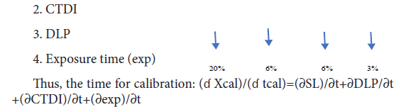
Three of the four scan parameters were within permissible limit and the major parameters that determine X-ray tube performance (CTDI and DLP) were found to be 6%. Scan length was not a major parameter since it does not affect CTDI and is dependent on the length of phantom and patient. Although, CTDI and DLP were within limit, there was variation in readings from preliminary to final due to the pitch factor (Tables 19 and 20). Thus, the time for calibration based on measurements should be at least twice per year.
| Scan Parameters | Average Percentage Difference | Permissible Limits |
|---|---|---|
| Scan Length | 20% | <± 10% |
| DLP | 6% | <± 20% |
| CTDI | 6% | <± 20% |
| Exposure time | 3% | <± 10% |
Table 20: Determination of calibration cycle; the table represents the percentage difference of scan parameters with time (duration of 1 year); The permissible limit is also illustrated according to IAEA and ACR standards. Three of the four scan parameters were within permissible limit and the major parameters that determine x-ray tube performance (CTDI and DLP) were found to be 6%. Scan length was not a major parameter since it does not affect CTDI and is dependent on the length of phantom and patient. Although, CTDI and DLP were within limit, there was variation in readings from preliminary to final due to the pitch factor. Thus, the time for calibration based on measurements should be at least twice per year.
Calibration Records
Percentage error (systematic and human)
The Exposure time, Pitch and fluence rate were the major parameters that vary CTDI and DLP. The CTDI and DLP was found to be 6% which was within permissible limits of IAEA standards (>± 20%). The optimum time for calibration should be at least twice per year for the GE Lightspeed Qxi CT unit based on the results obtained during the research.
Firstly, I (The researcher) would like to acknowledge Ms. Petal Surujpaul (Research Supervisor) and Dr. Sayan Chakraborty (Research Co-supervisor) for their technical and scientific contribution, motivation and support throughout the successful completion of the research.
Secondly, the researcher would like to show gratitude to Cancer Institute of Guyana for the access of the GE Lightspeed Qxi Computed Tomography Unit and Georgetown Public Hospital Corporation for the access of the Raysafe X2 CT Sensor.
Thirdly, I would like to acknowledge the staff of Cancer Institute of Guyana for their continued support and contributions during the practical aspect of the research.
Lastly, I wish to acknowledge my family who have supported and motivated me throughout the research.