International Journal of Advancements in Technology
Open Access
ISSN: 0976-4860
ISSN: 0976-4860
Research Article - (2022)Volume 13, Issue 9
In recent years, deep learning has almost invaded the world of telecom electronics and other fields, given the spectacular results it achieves in terms of improving the performance of digital processing chains. Wireless Access in Vehicle Environments (WAVE) technology has been developed, and IEEE 802.11p defines the Physical Layer (PHY) and Media Access Control (MAC) layer in the WAVE standard. However, the IEEE 802.11p frame structure, which has a low pilot density, makes it difficult to predict wireless channel properties in a vehicle environment with high vehicle speeds (high Doppler frequency), thus system performance are degraded in realistic vehicle environments. The motivation of this article is to improve channel estimation and tracking performance without modifying the IEEE 802.11p frame structure. Therefore, we propose a channel estimation technique based on deep learning that can perform well over the entire range of SNR values, the effects of ISI and ICI interference remain inescapable phenomena. The improvement brought by the LS channel estimation methods, MMSE and linear equalizers, cubic spline, linear DFT and cubic spline DFT interpolation are reviewed, these interpolation techniques contribute to the reduction of the BER in the chain. The different vehicular channel environment scenarios are split; simulations of the new estimation DNN method are performed on examples of high mobility channels, and compared to the LS and MMSE methods. A strong immunity of the proposed estimator against the high mobility of the channels is observed.
Channel estimation; Deep learning; Least Square (LS); Minimum Mean Square Error (MMSE); IEEE 802.11p standard; Vehicular channels
Orthogonal Frequency Division Multiplexing (OFDM) has invaded wireless communication due to its high data rate and capacity with high bandwidth efficiency and its robustness for multipath delay. It was used in wireless LAN standards such as the American communication standard IEEE802.11a and IEEE 802.11p in vehicular environments the dynamic channel estimation is performed before the demodulation of OFDM signals because the radio channel is frequency-selective and time varying for broadband mobile communication systems [1]. In recent years, deep learning has almost invaded the world of telecom electronics and other fields, given the spectacular results it achieves in terms of improving the performance of digital processing chains. Wireless Access in Vehicle Environments (WAVE) technology has been developed, and IEEE 802.11p defines the Physical Layer (PHY) and Media Access Control (MAC) layer in the WAVE standard. However, the IEEE 802.11p frame structure, which has a low pilot density, makes it difficult to predict wireless channel properties in a vehicle environment with high vehicle speeds (high Doppler frequency), thus system performance are degraded in realistic vehicle environments. The motivation of this article is to improve channel estimation and tracking performance without modifying the IEEE 802.11p frame structure. Therefore, we propose a channel estimation technique based on deep learning that can perform well over the entire range of SNR values, the effects of ISI and ICI interference remain inescapable phenomena. The improvement brought by the LS channel estimation methods, MMSE and linear equalizers, cubic spline, linear DFT and cubic spline DFT interpolation are reviewed, these interpolation techniques contribute to the reduction of the BER in the chain. The different vehicular channel environment scenarios are split; simulations of the new estimation DNN method are performed on examples of high mobility channels, and compared to the LS and MMSE methods. A strong immunity of the proposed estimator against the high mobility of the channels is observed.
In this paper, we study in section 2 channel estimation in thef physical layer of IEEE 802.11p. Standard channel model for wireless communication systems, in section 3 we describe all the traditional channel environment estimation methods and the proposed method based on DNN are presented in section 4. In section 5 all the simulations and the results and their interpretations finally section 6 concludes the article.
Channel estimation in IEEE 802.11p
In vehicular communications, reliable channel estimation of channels is considered a major critical challenge to ensure system performance due to the extremely time-varying characteristic of vehicular channels. The main challenge is to follow the channel variations over the length of the packets while respecting the standard specifications. Figure 1 specifies the comb-type driver arrangement in IEEE 802.11p [2]. This layout consists of two types of drivers: block and comb drivers. The figure shows the principle of Least Squares (LS) estimation based on block pilots, which are executed first to obtain the response channel frequency. Such LS appreciates limits performance due to rapid channel variations and sparse block driver placement. To overcome this problem, pilots must be periodically added to the data network to provide channel updating and tracking, after which the initial insertion correlation in the time and frequency domains can be exploited to improve the performance of Estimate of the channel. Accordingly, after performing the initial LS estimation on the block pilots in [3], linear filtering of the minimum Mean Squared Error (MSE) in the time domain was implemented on the comb pilots to track the channel change over time, given
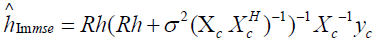

Figure 1: Group-three clustering cell.
Where Rh=E (h hH) is the channel time domain correlation matrix, XC is the pilot training comb, yc is the received signal, and σ2 is the power noise. For WSSUS environments, the correlation of channel frequency responses at different times and frequencies [4], rH (Δt, Δf) can be decoupled as the product of that in the time domain, rt (Δt), and that in the frequency domain, rf (Δf), i.e. rH (Δt, Δf)=rt (Δt) rf (Δf) where rt (Δt), depends on the speed of the vehicle or, equivalently, the Doppler shift and rf (Δf), depend on the multipath delay propagation channel estimation based on block pilots. Channel block, there will be no channel estimation error since pilots are sent on all carriers. Estimation can be performed using LS or MMSE. If inter symbol interference is eliminated by the guard interval, the problem is how, where and how often to insert pilot symbols. The spacing between pilot symbols must be smaller to make channel estimates reliable. to determine the number of pilot tones needed, the frequency domain channel transfer function H (f) is the Fourier transform of the impulse response h (t). Each of the impulses in the impulse response will result in a complex exponential function T in the frequency domain, given its delay where is the symbol time. sampling this contribution to H (f) assumes compliance with Nyquist sampling theorem and the maximum pilot spacing, Δ f in the OFDM symbol is: Δp ≤ (NTSΔf)/2τ where N is the number of subcarriers, Δf is the Doppler shift TS=8 μs is the symbol duration OFDM. The channel can be estimated at pilot frequencies in two ways: LS and (LMMSE). For block type arrangements, the pilot tone channel can be estimated using LS or MMSE estimate, it also assumes that the channel remains the same for the whole block. MMSE estimate gives 10-12 dB gain in Signal-to-Noise Ratio (SNR) on the LS estimate for the same root mean square error of the channel estimate. Comb type pilot tone estimation was introduced to meet the need for equalization when the channel changes even in an OFDM block. Channel estimation at pilot frequencies for channel estimation based on comb type can be based on LS, MMSE or Least-Mean-Square (LMS) MMSE works much better than LS. For study Principe of LS estimate see appendix 1 in comb type pilot arrangement, pilot symbols are inserted into sub-carriers with same interval. This type of pilot arrangement is suitable when channel conditions change from one OFDM block to the subsequent one. If NP are numbers of pilot signals then X (k) can be written as:
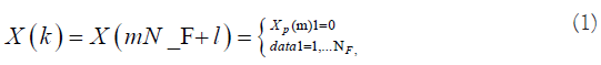
Where X (k) is the information, including pilots and data of all sub-carriers, Xp (m) is the mth pilot carrier value and NF represents frequency interval of inserted pilots (NF=NFFT/NP). According to the pilot positions, frequency response of corresponding sub- channel is calculated in the receiver.
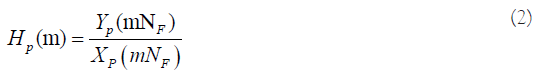
After estimating the channel transfer function Hp (m) from pilot tones, an efficient interpolation method is applied on pilot sub- carriers and obtained NFFT points channel transfer function H (k).
Linear interpolation
Linear interpolation is also a simple method. It consists, for data subcarrier km GI ≤k ≤ (m+1) GI, the estimated channel response using linear interpolation is given by:

The linear channel interpolation can be implemented by using digital filtering such as Farrow-structure. Furthermore, by carefully inspecting equation, we find that if GI is chosen as power of 2, the multiplications operations involved in equation can be replaced by shift operations, and therefore no multiplication operation is needed in the linear channel interpolation. GI=N/Np, N is the number of subcarrier, Np number of pilot It is obvious to notice that this method of interpolation is clearly better than that of the nearest eighbor. In addition, we notice that this method offers bad results when the channel is very selective in frequency.
Spline cubic interpolation
Method gives smooth and better interpolation accuracy but the performance improvement is not obviously proven. It uses higher order interpolation. Spline cubic interpolation is representented as in Figure 2 the expression of the interpolated channel is given by:


Figure 2: Spline cubic interpolation method. Note:  Pilot,
  Data,
Data,  Interpolations.
IEEE 802.11p standard
AThe Intelligent Transport System (ITS) is one of many viable solutions to improve road safety, where the means of communication (e.g., between vehicles and between vehicles and other components of and ITS environment, such as road infrastructure) are usually wireless. The typical communication standard adopted by car manufacturers is IEEE 802.11p. Thus, this article presents an inventory of the IEEE 802.11p, more precisely, we analyze the MAC and PHY layers in an environment Dedicated to Short-Range Communications (DSRC) by studying the limitations of the chain and we propose the solutions. To improve the efficiency of the wireless transmission chains used in this standard.
Criterion of the IEEE 802.11p standard: For vehicular communications, the IEEE 802.11a standard [5] has been modified by the P working group (TGp) to give birth to the IEEE 802.11 standard p. It uses the physical layer (OFDM) (previously specified in IEEE 802.11a IEEE 802.11p specifies a set of parameters for the physical layer (PHY), dealing with vehicle scenarios. OFDM is a modulation technique in which the bandwidth of overall transmission B is subdivided into N orthogonal B/N band subcarriers. Each subcarrier is subject to flat frequency fading, allowing simple channel equalization on the receiver side. To (ISI) avoid intersymbol interference; OFDM implements a specific form of guard period, the cyclic prefix. The cyclic prefix is a copy of the last G samples from the end of the OFDM symbol. To implement OFDM, a Discrete Fourier Transform (DFT) is computed with Tx and Rx. In addition to efficient DFT using the fast fourier transform. For OFDM system design, two basic wireless channel parameters must be considered: Excess delay fmax and the doppler spread fD. Excessive (maximum) sets a limit to the maximum data rate that can be used without an equalizer, or similarly it determines the minimum duration of the cyclic prefix in OFDM.

The Doppler spread determines the minimum subcarrier spacing in OFDM systems before the onset of inter carrier interference, due to loss of Subcarrier orthogonality.

As additional constraint the spectral efficiency

Shall be as large as possible for coherent detection, Channel State Information (CSI) is required. To obtain CSI, current standards rely on known pilot symbols that are interleaved with the data in the OFDM time-frequency grid. For the system design it is crucial to place the pilot symbols in the OFDM time-frequency grid according to the maximum excess delay and the doppler spread of the wireless communication channel. The maximum excess delay determines how dense pilot symbols must be transmitted in frequency domain, and the maximum pilot spacing f (number of subcarriers) will satisfy.

The Doppler spread determines how dense pilot symbols must be placed in time. The maximum spacing t (number of OFDM symbols) will satisfy.

Specific choices of OFDM parameters allow for a wide range of applications from broadcasting [6] to cellular [7], WLAN [8], and vehicular connectivity [9].
IEEE 802.11p system performance: Ensure that the cyclic prefix length G=16 corresponding samples corresponding to a tolerable excessive delay of 1.6 μs corresponding to a distance at a propagation distance of 480 m. 802.11p bandwidth reduced to 10 MHZ With N=64 subcarriers, only 52 are used due to guard band
requirements. The performance of the 802.11p system is largely determined by the receiver’s channel estimator and channel equalizer. the estimation and equalization techniques of the IEEE 802.11a model are the same as those used in IEEE 802.11p this type of driver is well suited for mobile indoor use, but not for vehicular scenarios where the channels are jointly time-selective frequency. Which leads to a loss of performance if too naive channel estimators are used the IEEE 802.11p driver model uses two types of drivers: 1) block drivers and 2) comb drivers. The 52 subcarriers of the first two OFDM symbols are dedicated to the pilots. In the remaining OFDM symbols, only four subcarriers contain pilots for the entire duration of the frame two types of estimators exist; block type channel estimator: a channel estimate is calculated from block pilots only. The estimated channel coefficients are used for the whole frame the LS estimator is used SEE appendix a.
Block-comb channel estimator: First, the temporal correlation function is estimated using the comb pilots. Subsequently, a linear Minimum Mean Squared Error (MMSE) filtering structure requires greater complexity than the LS estimator to allow for the temporal variance of the channel. Acceptable performance is expected for short block lengths, as well as for channels with short delay spread and high doppler spread, or high delay spread but low doppler spread. Conversely, under NLOS conditions with a Doppler spread fD>500 Hz and a maximum delay max>400 ns, performance losses are unavoidable. The objective of this work is. to verify that the limitations of classical LS OR MMSE estimation methods, for certain channel scenarios, are easily overcome by using DNN-based estmators for this we will take some environments giving worse performance with the classical methods that we try with the estimation based on DNN transmission fidelity BER were found.
Environment and vehicular channel
DSRC robustness to doppler spread is a concern for faster applications. The surrounding environment was very varied due to the presence of hills, bridges and other concrete structures. Traffic was also uncontrolled, with a mix of passenger vehicles and large tractor-trailer trucks. Non Line of Sight (NLOS) conditions were created either by terrain or by the imposition of blocking vehicles (e.g. large trucks or towed trailers) between our transmitter and receiver. LOS test locations. When LOS is present, freeway scenarios are characterized by short delay gaps but potentially large doppler gaps. Highway speeds were about 30 m/s and the carrier frequency of the waveform was 5900 MHz. Thus, doppler shifts of 1.1 kHz or more are possible when reflections from obstacles directly in front of the transmitter and receiver are taken into account. For example, a reflection off a bridge crossing the road (i.e. an “overpass”) gives an effective path closure rate of 60 m/s and a doppler shift of 1172 Hz reflections off vehicles in approach (also moving at 30 m/s) lead to an approach speed of 120 m/s and a doppler shift of 2.3 kHz. doppler spread represents a range of reflections from many angles (and therefore different closure rates), spreads greater than 2 kHz are possible, the different scenarios are summarized.
Vehicular channel modeling
The effects of channel propagation in vehicular communications differ from those in wireless systems. Vehicular channels have rapid temporal variability and inherent non-stationarity in channel statistics due to their unique physics dynamics of the environment [10]. Therefore, an appropriate mathematical modeling for the vehicular channels is essential to evaluate their effects in the transmission chain. Let denote the distance in meters between the transmitter and receiver.
Path loss in vanet
To predict the received signal strength in the Line-of-Sight (los) environment or the free space propagation model is let d be the distance in meters.
Between transmitter and receiver when non-isotropic antennas are used with a transmitter gain of Gt and a reception gain of Gr, the power received at a distance, is expressed by the Friis equation given by Pr (d)=(Pt Gt Gr λ2)/(4π)2 d2L) (2.11) where Pt is the transmit power (watts), λ is the radiation wavelength (m), and L is the system loss factor which does not depend of the propagation environment. It represents the overall attenuation or loss in the actual system hardware, including the transmission line, filter, and antennas. Typically L>1, L=1 assuming no loss in system hardware. It follows from equation (2.11) that the received power attenuates exponentially with distance d. the free space path loss PLF (d) without any system loss, can be directly derived from equation (2.11) environment, the free-space path loss PLF (d), without any system loss can be directly derived from equation (2.11)
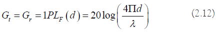
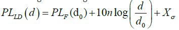
for the IEEE 802.11 p standard, the free space path loss at the carrier frequency fc of 5.9 GHz for different antenna gains diminished and when the distance separating the transmitter and the receiver d increases, as shown in the Figure 3. A more generalized form of the path loss model can be constructed by modifying the free space path loss with the path loss exponent which varies by environment. This is known as the log-distance path loss model, in which the distance path loss d is given as evidence that the path loss increases by reducing the antenna gains PLLD (d)=PLF (d0)+10nlog (d/d0) (1.13). A d0 must be correctly determined for different propagation environments. Show the value of n for different environment. Note that n=2 correspond to the free space. Moreover tends to increase as there are more obstructions (Figure 4).

Figure 3: Free-space path loss in vanet. Note:  Gt-1.Gr-1,
  Gt-1.Gr-0.5,
  Gt-0.5.Gr-0.5.

Figure 4: Log-distance path loss model. Note:  n=2,
n=2,  n=3,
n=3, n=6.
n=6.
Shadow-fading models
It is clear that the path loss increases with the path loss exponent. Even if the distance between the transmitter and receiver is equal to each other, every path may have different path loss since the surrounding environments may vary with the location of the receiver in practice. However, not all the aforementioned path loss models consider this particular situation. A lognormal shadowing model is useful when dealing with a more realistic situation. Let Xσ denote a Gaussian random variable with a zero mean and a standard deviation of σ. Then, the log-normal shadowing model is given as:
Alternatively, this particular model allows the receiver at the same distance to have different path loss, which varies with Xσ random shading effects. Figure 5 shows the path loss that follows the log- normal shadowing model at fc=5. 9GHz with σ=3 dB and n=2. It clearly illustrates the random effect of shadowing that is imposed on the deterministic nature of the log-distance path loss model. The results clearly show that the log-normal shading introduces randomness into the received signal power, which can bring us closer to reality [11].

Figure 5: Log normal shadowing path loss model. Note:  Log
normal shadowing,
Log
normal shadowing,  First model.
Determinist model of v2v channel
Small-scale fading occurs over distances from the carrier wavelength due to the construction and destructive effects of multiple time-varying delayed aftershocks original signals received from different paths between the transmitter and the receiver. The time-varying channel impulse response can be expressed as follows:

Where γi denote the complex amplitude, τi is delay and Φi (t)=2πfc τi (t)-φνl, where φνl=∫ 2π fνl dt is the phase that depends on the delay and doppler of the lth multi-path component MPC at time t, respectively. In time variant systems it is important to distinguish between the delay τ and the absolute time t over their way the general expression (1.1) represents a doubly selective channel since there are several paths and the attenuations and delays are a function of time two examples s for h (t,τ) are used.
Time-invariant frequency-selective channel: When the transmitter, receiver, and surroundings are stationary, the attenuations γi (t) and the deadlines for propagation τi (t) do not depend on time. However, the delays are significantly large compared to the period of the symbol. Figure 6 gives an example for velocity v=2 km/h.

Figure 6: Doppler effect in times domain for the vanet channel.
Time-varying (or time-selective) flat-fading channel: The delays τi (t) is approximately constant and small compared to the symbol period. This scenario occurs when the transmitter or receiver is mobile and when the symbol the period of the transmitted signal greatly exceeds one of all the delays. Since the symbol period TS decreases when the data rate increases, the channel may be flat or frequency-selective fading depending on the data rate. The delay spread is another relevant parameter delay spread.

TS>>Td we defined also BC=1/5Tram=1/Tmax, (3.3) channel fades flat. Otherwise, the channel is frequency selective. As an example the typical delay propagation in a wireless channel in an urban area is 5 μs when the distance between transmitter and receiver is 1 km for data rate is 1 kbps, 1 ms and the channel is faded flat because Td<< Ts. for a debit of 1 Mbps, Ts is 1 μs the channel becomes frequency selective because Ts<<Td the mobility of the transmitter or the receiver will induce a change of radiofrequency, called Doppler shift Ds. TC coherence time, one parameter Linked to the Doppler shift by:

If the coherence time TC is comparable to the symbol period, the channel is time-varying. In contrast, in time-invariant channels, the coherence time TC is much larger than the period of the symbol i.e. the channel remains constant. As an example, DS=54.62 Hz given if v=2 km/h and the transmit data rate is 1 Mbps, then TC=9.145ms is much greater than 1 μs symbol duration. Another value for DS=2185.18 Hz for v=400 km/h and the transmit rate is 1Mbps then TC=0.228 ms less than the 1 ms symbol duration if the transmit rate is 1 kbps, Figures 2 and 3 shows the effect of the doopler effect for the vanet channel it gives this type of channel for velocity v=120 km/h and 400 km/h this is a time varying channel. Figure 7 shows how the amplitude of the first path of the channel varies according to the speed of the mobile, so the doppler effect on the behavior of the channel we find the behavior of the two types of channel already mentioned. The types of wireless channels are depicted in Table 1.
| Environment | Path loss exponent (n) |
|---|---|
| Free space | 2 |
| Urban area cellular radio | 2.7-3.5 |
| Shadowed urban cellular radio | 3-5 |
| In building line-of-sight | 1.6-1.8 |
| Obstructed in building | 4-6 |
| Obstructed in factories | 2-3 |
Table 1: Give value of n for different environment.

Figure 7: Doppler effect in first path weakening for jakes model
channel. Note:  Mobile velocity=10 km/h,
  Mobile
velocity=100 km/h,
Mobile
velocity=100 km/h,  Mobile velocity =500 Km/h.
Statistical channel parameters
The impulse response of the time-varying CIR channel: h (τ, t) is usually estimated via the measured power Delay Profiles (PDP).
The most common PDP statistic is RMS delay deviation, τrms. H
(f, t) is the fourier transform of h (τ, t) with respect to τ. The
Spaced-Frequency, Spaced-Time (SFST) correlation function:
R (t, f, Δt, Δf)=correlation of time variation TF, to time shift
Δt, frequency separation Δf. When the scattering at different
delays is uncorrelated and the time variation is broad-sense
stationary, this reduces to R (Δt, Δf). The width of R (Δt, Δf)
is called coherence, or correlation, bandwidth, Bc, which is a
measure of correlation between channel effects at two different
frequencies. As a rule, we have  The width of R (Δt,
0) is the coherence time, TC. Diffusion function SF: S (t, f, υ,
τ)=average channel output power as a function of delay τ and
doppler, this is the double fourier transform of R (t, f, Δt , Δf) =
correlation of the variable time TF, at the time shift Δt, frequency
difference Δf in case of uncorrelated scattering and broad-sense
stationarity, SF reduces to S (υ, τ), double Fourier transform of
R (Δt, Δf). The approximate width of S(υ, τ) in υ is the Doppler
spread fd=1/TC. The corresponding function simultaneously
observes the dispersion provided by the channel in the time and
frequency domains, hence its name: delay-doppler dispersion
function. The dispersion function combines information about
doppler shifts and path delays. The basic idea behind dispersion
functions is that they plot expected power by doppler shift and
excessive delay each path can be described by its Angle of arrival
and doppler shift Excessive delay. Thus, we can plot the received
energy in a two-dimensional plane, with a Doppler shift on one
horizontal axis and a delay on the other horizontal axis example
consider a u-shaped doppler spectrum, as it occurs with uniformly
distributed angles of arrival of reflected waves. The maximum
offset is fm. an exponential delay spread of average Trms. Moreover,
we assume that the delay spread and the doppler spread are
separable. Then the amount of (broadcast power) per frequency
and time slot can be expressed as:
The width of R (Δt,
0) is the coherence time, TC. Diffusion function SF: S (t, f, υ,
τ)=average channel output power as a function of delay τ and
doppler, this is the double fourier transform of R (t, f, Δt , Δf) =
correlation of the variable time TF, at the time shift Δt, frequency
difference Δf in case of uncorrelated scattering and broad-sense
stationarity, SF reduces to S (υ, τ), double Fourier transform of
R (Δt, Δf). The approximate width of S(υ, τ) in υ is the Doppler
spread fd=1/TC. The corresponding function simultaneously
observes the dispersion provided by the channel in the time and
frequency domains, hence its name: delay-doppler dispersion
function. The dispersion function combines information about
doppler shifts and path delays. The basic idea behind dispersion
functions is that they plot expected power by doppler shift and
excessive delay each path can be described by its Angle of arrival
and doppler shift Excessive delay. Thus, we can plot the received
energy in a two-dimensional plane, with a Doppler shift on one
horizontal axis and a delay on the other horizontal axis example
consider a u-shaped doppler spectrum, as it occurs with uniformly
distributed angles of arrival of reflected waves. The maximum
offset is fm. an exponential delay spread of average Trms. Moreover,
we assume that the delay spread and the doppler spread are
separable. Then the amount of (broadcast power) per frequency
and time slot can be expressed as:
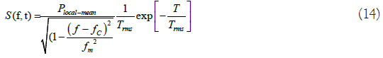
Appendix B gives the theoretical foundations of this type of channel. The function S (τ, ν), this function is simulated for two types of channels VTV Expressway (VTV-EX) and RTV- UC: Described in Tables 2 and 3 to describe the channel, we use the statistical function denoted shy, and function 1/τrms exp (-τ/ τrms) can is easily derived from the functions previously defined with the following relation’s (Δf): Where, P(local-mean) is the received power level averaged over an area of tens or hundreds of meters fc=5.9G Hz is the carrier frequency used in IEEE 802.11p, fm is the maximum doppler frequency defined in Table 2 for each channel type. The following script plots the given diffusion function as a 3D plot. It also plots the power delay profile and the doppler power spectrum by projecting the 3D plot along the x-axis and the y-axis represents this function for two types of v2v channel, Figure 8 gives the channel characteristics RTV-SS channel for τrms=21.6 ns, fd=580 Hz (v=30 km/h), Figure 9 gives the characteristic of the channel VTV-EX channel. By making a simulation comparison, it can be seen that the power of the received signal degrades significantly when the doppler frequency increases.
| Environment link type | Highway σ (dB) | Urban σ (dB) |
|---|---|---|
| LOS | 3.3 | 5.2 |
| Nosh | 3.8 | 5.3 |
| Lobs | 4.1 | 6.8 |
Table 2: Shadow-fading parameter for V2V communication.
| Type of channel | Conditions and characteristics |
|---|---|
| Time varying | Tc<<Ts |
| Time invariant | Tc>>Ts |
| Flat fading | Td<<Ts |
| Frequency selective | Td>>Ts |
Table 3: VANET channel parameter and configuration.

Figure 8: Scattering function, power delay profile and doppler power spectrum for RTV UC channel for Trms=21 ns, fd=207 Hz (v=104.4 km/h) fc=5.9 GHz.

Figure 9: Scattering function, power delay profile and doppler power spectrum for VTV-EX channel for Trms=774.58 ns, fd=1280 Hz, fc (v=235 km/h)=5.9 GHz.
This is the reason to think about the new method of channel estimation to compensate for these channel effects for τrms=774.58 ns, fd=1280 Hz (v=278 km/h) fc=5.9 GHz detailed channels Study the response of the responses of the two channels.
Environment comparison
Examination of Table 4 pull in suggests that the proposed design parameters for 802.11p are met [12]. A first examination of Table 1 we can see that .the guard interval is 1.6 μs is less than the propagation delay T ̅ and τrms can deduce that the phenomenon of intersymbol interference ISI does not exist for all the scenarios of the ISI website. For 802.11p, this Guard Interval (GI) is 1.6 μs, twice as long as the 802.11a IG of 0.8 μs for an OFDM transmitter to insert a small number of pilot tones into a symbol of data for DSRC.
| Environment | Separation (m) | T (ns) | Tram (ns) | Tmax (ns) | Coherence time (µs) | Ds (hz) |
|---|---|---|---|---|---|---|
| High loss | 00-50 RTVUC | 69.18 | 21.06 | 349.43 | 880.46 µs | 567.88 |
| 50-200 | 208.21 | 95. 02 | 1227.22 | 184.21 µs | 2714.29 | |
| 200-00 | 163.63 | 112.33 | 1527.22 | 328.86 µs | 1520.39 | |
| >500 | 119.39 | 50.88 | 924.24 | - | 1248.6 | |
| Overall | 117.58 | 54.06 | 778.79 | - | 1223.99 | |
| High N loss | 00-150 | 266.65 | 267.65 | 5939.39 | 147.84 µs | 3382.01 |
| 150-300 | 255.66 | 136.59 | 1575.76 | 133.33 | 3750.94 | |
| >300 | 293.01 | 379.58 | 6109.06 | - | 3289.93 | |
| Overall | 268.19 | 238.83 | 4152.11-284.49 | - | 3515.03 | |
| Urban loss | 0-75 VTV-EX | 281.15 | 774.58 | 10870.1 | - | 1270.35 |
| 75-150 | 268.27 | 247.66 | 3347.11 | - | 2309.4 | |
| 150-50 | 330.32 | 430.25 | 5232.32 | - | 2236.47 | |
| 250-350 | 259.68 | 232.15 | 3188.55 | - | 1700.61 | |
| 350-450 | 330.00 | 281.26 | 3396.36 | - | 1918.13 | |
| >450 | 439.38 | 726 | 10933.3 | - | 2533.66 | |
| Overall | 312.17 | 436.74 | 5973.06 | - | 3515.03 | |
| Urban NLOSS | 0-150 | 378.6 | 227.26 | 1739.39 | - | 2674.21 |
| 150-250 | 451.02 | 368.84 | 2174.25 | - | 950.23 | |
| 250-500 | 490.8 | 406.63 | 2310.61 | - | 1146..29 | |
| 500-800 | 366.82 | 402.33 | 2370.61 | - | 491.92 | |
| 800-1000 | 319.47 | 343.87 | 2227..21 | - | 478..04 | |
| >1000 | 236.99 | 249.25 | 1765.5 | - | 439.24 | |
| Overall | 375.52 | 329.38 | - | - | 1043.48 | |
| Rural los | 0-120 | 85.84 | 145.29 | 3125.87 | - | 783.63 |
Table 4: Technical characteristics of the different types of vehicular channel.
The symbol contains four pilots spaced 2.1875 MHz apart (14 subcarriers). Based on an inverse relationship between coherence time and delay spread should not be greater than about 457.14 ns. Only highway LOS and coherent rural LOS environments need to have sufficiently large coherence bandwidth. Highway NLOS has an average delay propagation sum of 507.02 ns (1.972 MHz), while urban LOS/NLOS environments are at 748.91 ns (1.335 MHz) and 704.9 ns (1.419 MHz), respectively. Therefore more complex equalization algorithms, such as pilot interpolation schemes, should be considered as alternatives to flat-fading corrections in these environments. Similarly, the standard takes into account some doppler deficiencies but not others. Induced doppler shifts can cause an ICI between OFDM subcarriers. However, from the table we see that the highest mean doppler deviation is 3750.94 Hz for the case of the NLOS 150- 300 m highway. This is a small fraction (2.40%) of the 156.25 kHz intercarrier spacing for 802.11p. In fact, it was rare to see a channel price with a Doppler spread of 2 kHz, or only 1.28% of the intercarrier spacing. Therefore, even under the most dangerous Doppler conditions, the amount of ICI should be minimal.
Structure of the DNN implants network
An Orthogonal Frequency Division Multiplexing (OFDM) communication system is given in Figure 10. On the transmitter side, the source bits X (k) drive the modulation operations, Inverse Discrete Fourier Transform (IDFT) and Cyclic Prefix Addition (CP), respectively. Denote the multipath fading channels as h (0), h (1), h (L-1). The signals are transmitted over the channel, which is generally dispersive. Express the discrete sample spacing multipath channel as (h(n))n=0 N-1, where the random variable h (n) is the gain of the channel at time n. this channel gain will represent the core of this work as the idea is to implement DNN estimators for channels representing most scenarios of the vehicular channel (see Table 1 section), the receiver signal is Y (n)=x(n) ⊗ h (n)+w (n), (19) where x (n) and w (n) denote transmitted signal and noise respectively, and ⊗ represent circular convolution. After removing CP and DFT operation, the received signals can be obtained as Y (k)=X (k) H (k)+W (k) (20) où Y (k), X (k), H (K) et W (k) are the DFTs of y (n), x (n), h (n) and w (n) respectively. Finally, source information is recovered from Y (k) through domain frequency equalization and demodulation generally, the traditional.

Figure 10: System model for OFDM with DNN based equalizer.
OFDM receiver first estimates the CSI H (k) using the driver, and then detects the source signal with the estimated channel Hˆ(k), a method based on transceiver deep learning is which can estimate CSI implicitly and recover the signaler directly. This approach considers the whole receiver as a black box, takes the signal received as input from a Deep NN (DNN), and outputs the source bits recovered after calculation and transformation in the hidden layers of the NN. An OFDM frame is composed of two blocks: One representing the pilot symbols and the other for the data. The channel parameters remain in each frame and may vary between frames. The 64 sub-carriers and the length of CP is 16. The first block is used in each frame, the fixed pilot symbols, and the second data block is composed of 128 random binary bits. After QPSK modulations, IDFT and CP insertion, all donations frame data are convolved with the channel vector. This channel vector will be simulated by a matlab channel function, which will represent all the main vehicular communication scenarios, the simulation parameters are fixed in Table 2. On the receiver side, the received signals, including noise and interference in the frame will be collected as DNN entry after CP removal. The DNN model aims to learn the parameters of the wireless channel to be able to recover the source signals. As shown in Figure 11, the architecture of the DNN model is composed of five couches: input layer, three hidden couches, and output layer. The number of neurons in the input layer is 256 since the real and imaginary parts are processed separately. The number of neurons in the three hidden layers is 500, 250 and 120 respectively.

Figure 11: DNN architecture.
Simulation and resultants
Linear interpolation LS Cubic spline interpolation LS Linear interpolation Linear spline interpolation Cubic interpolation DFT the simulation parameters are Given in Table 5 In Figure 12 we compared for the LS estimator the different linear, cubic spline, and cubic spline (DFT) interpolation methods [13]. It is noticed that the cubic spline interpolation methods (DFT) give the best results (low BER) compared to the other methods results in comparison with other methods.
| Parameters | Specifications |
|---|---|
| FFT size | 2048 |
| Number of active subcarriers | 2560 |
| Pilot ratio | 1/4 |
| Guard interval | 16 |
| Guard type | Cyclic prefix |
| Chan.path delays (s) | [0.0, 0.2,0.5, 1.6, 2.3, 5.0]* 1e-6 |
| Chan.avg path gain dB | [-3, 0, -2, -6, -8, -10] |
| Channel type | Rayleigh RTV-UC |
| Doopler frequency shift (hz) | 3382 |
Table 5: Parameter of simulation of classic estimators.

Figure 12: Comparing MMSE and linear interpolation and spline cubic interpolation. Note:  LS-linear
interpolation,
LS-linear
interpolation,  LS-spline cubic interpolation,
  MMSE.
MMSE.
According to Figures 13 and 14 (LS and MMSE) can be improved with the incorporation of the DFT AND SPLINE algorithm. The improved channel estimation with the DFT algorithm has been achieved by removing the noise impact outside of the maximum channel delay length. we retain the best performance presented by the MMSE estimator (low BER) compared to the other estimation methods presented in Figure 14, the one whose performance is the weakest is the LS method, the new estimation method based on the deep-learning channel estimation methods In this simulation, in Figure 15 the cyclic prefix effect is studied here cp is taken as zero length of the cyclic prefix is less than the maximum average delay propagation of the channel 350 ns, equalization fails for LS and MMSE estimators by setting cp=16 the length of the cyclic prefix of 16.8 μsec is greater than the maximum average delay propagation of the channel, equalization succeeds with the dnn estimator with cp or without cp gives better performance a than the classic LS and mmse estimators with cp , another strong point of the deep learning method (Table 6).
| Parameter | Value |
|---|---|
| Number of subcarriers | 64 |
| Number of pilot | 16 |
| Signal modulation | QPSK, 16 QAM |
| Cyclic prefix | 16 |
| Channel model | RTV-SS and VTV-EX |
| Number of path | 12-11 |
| Input number of hidden layes | 160,260,360 |
| Number of neurons | 3 |
| Epoch number | 100 |
| Training function | Softmax relu |
| Gradient threshold | 10 |
| Learn Rate Drop Factor | 0.1 |
| Optimization algorithms | SGDM, Adam |
| Doppler frequencies (hz) | 5, 500, 1200, 2000 , 2500, 3500 |
Table 6: DNN parameter estimator.

Figure 13: Performance of LS spline cubic interpolation (DFT). Note:  LS-linear interpolation,
  LS-spline cubic interpolation,
  MMSE,
MMSE,  LS-spline cubic interpolation (DFT).

Figure 14: Impact of the cp RTV-UC channel. Note:  Without CP-DL,
  With CP-DL,
  Without
CP-LS,
Without
CP-LS,  Without CP-MMSE.

Figure 15: BER in Qpsk CP=16, RTV-UCfd=207 Hz. Note:  Deep Learning (DL),
  Least Square (LS),
  Minimum Mean Square Error (MMSE)
Channel’s coherence time effect
Table 6 propose the main parameters used to validate the results of the proposed estimation method based on deep learning called DL estimator, especially at low values of SNR, FIR URE 16 illustrates the performance of the bit error rate of the DNN method and the traditional estimators: LS and LMMSE. It can be seen that the LS method is the least efficient and that the DNN method has the same performance. One of the proposals made in this work is to validate the non-limitation of the estimator based on the DNN in the face of the high mobility present in the vehicular channel because these several examples of channels have been tested with the DNN approach the channel taken is the next delay=(0, 1, 2, 100, 101, 200, 201, 202, 300, 301, 302)*1e-9s; powderd B=(0, 0, 0, -6.3, -6.3, -25.1, -25.1, -25.1, -22.7, --22.7, -22.7), and the doppler frequencies are 5 hz, 207 hz, 500 hz, 1200 hz, 2500 hz, 3000 hz, 3500 hz. The curves in Figure 16 representing the results in terms of BER against the LS and mse estimators are given in the figures clearly the DNN estimator offers better results low BER when the channel is more and more mobile (when fd increases) as seen in the Table 7 In this simulation, the coherence time effect of channel is studied. The channel coherence time must be large enough for each symbol to be visible channel. The symbol time TS=8 μs is less than the coherence time of the channel given in equation (3.4), representing the different scenarios described in Table 2 therefore the equalization is successful (because the entire symbol sees the same non-variable channel). In Table 7, we study the impact of the doppler shift. These results show that the variations on the channel statistics models degrade the performance of the LMMSE estimator, but have no significant influence on the performance of the DL based estimator. These results also validate the excellent generalizability of the DL-based estimator with respect to the maximum doppler frequency.
| Snr dB | 0 | 2 | 4 | 6 | 8 | 10 | 12 | 14 | 16 | 18 | 20 |
|---|---|---|---|---|---|---|---|---|---|---|---|
| Dl BER Fd=3500 hz |
0,6174 | 0,5633 | 0,4803 | 0,3925 | 0,2921 | 0,1845 | 0,101 | 0,0451 | 0,01340 | 0,00219 | 9.99 e-05 |
| Dl BER Fd=3000 hz | 0.6193 | 0.5588 | 0.4834 | 0.3882 | 0.2891 | 0.1487 | 0.0146 | 0.0013 | 0.0013 | 3.00E-04 | 0 |
| Dl BER Fd=2500 hz |
0.6102 | 0.566 | 0.4924 | 0.3999 | 0.2914 | 0.1925 | 0.0955 | 0.0432 | 0.0104 | 0.0022 | 3e-4 |
| DL BER Fd=500 hz | 0.6157 | 0.56560 | 0.4877 | 0.4018 | 0.2935 | 0.2935 | 0.1011 | 0.0412 | 0.0123 | 0.0016 | 9.1e-04 |
| Dl BER Fd=5 hz |
0.6026 | 0.5611 | 0.9464 | 0.3983 | 0.2936 | 0.1843 | 0.1017 | 0.0417 | 0.120 | 0.0033 | 0 |
Table 7: Doppler effect in BER of the estimator DNN.

Figure 16: BER in Qpsk VTV-Ex Channel CP=16 and different value of fd (a, b, c, d, e, f). Note:  Deep
Learning (DL),
Deep
Learning (DL),  Least Square (LS),
  Minimum Mean Square Error (MMSE)
Effect of modulation scheme
Two types of modulations are tested qpsk and 64 qam. The same parameters are used and the comparison of the performances of the two methods is presented in Table 5, at constant BER The SNR of DL is lower than that of the LS and MMSE algorithms, in particular in QPSK, the DL maintains good signal detection in a highly mobile channel. The detection performance of the LS and MMSE algorithms is less affected by the modulation mode, but the detection accuracy is low. Increasing M for MQAM modulation gives better results but complicates the system on the implementation side (Table 8).
| SNR Qpsk | SNR 64 QAM | |
|---|---|---|
| LS | 19.1 dB | 21 B |
| MMSE | 19 dB | 20 B |
| DL | 13 dB | 18 B |
Table 8: Comparison SNR for QPSK and 64 QAM for LS MMSE and DL estimator with fixed ber=510-3.
Effect of optimization algorithms
On the performance of the proposed estimator optimization algorithms play a vital role in improving DL processes. The formation of deep neural networks can be described as an optimization problem that seeks to find a global optimum thanks to a reliable formation trajectory and rapid convergence using gradient descent algorithms. The purpose of a DL process is to find a model that will produce better and faster results thanks to weights and biases adjusted to minimize loss function (gradient descent). Choose the optimal optimization approach for a scientific problem acts as a serious challenge. Choosing an inappropriate optimization approach can cause the network to reside in the local minima during training, and this does not reach any progress in the learning process presents an experimental comparison of the performance of two optimization algorithms SGDM and ADAM [14]. It will also study to what extent each optimizer can deal with the problem of channel state estimation; therefore find the most effective CSE the three optimization algorithms used are Adam, SGDM. The effectiveness of the SGDM learning process to obtain a more reliable DNN-based CSE will be investigated. It is evident from Table 9 that the SGDM models outperform the Adam models at 64 pilots.
| Snr dB | 0 | 4 | 10 | 14 | 18 | 20 |
|---|---|---|---|---|---|---|
| SER DL | 0.619 | 0.487 | 0.187 | 0.041 | 0.0019 | e-4 |
| SGMD | ||||||
| SER DL | 0.614 | 0.4903 | 0.183 | 0.0404 | 0.0125 | 0 |
| ADAM |
Table 9: SGDM and Adam optimization algorithm comparing.
In this article, a method based on deep learning is the estimation of the vanet channel, the latter gives good results in terms of low BER error rate and a strong robustness with respect to the different phenomena of non- linearity present in siso OFDM chain. A vanet channel model is proposed covering the low mobility channels up to the high mobility channel. Interesting results are obtained on the DL method for a vanet channel in comparison with the classical methods for the same type of channel and a strong vis robustness. The various non-linearity phenomena present in the siso OFDM chain, we retain the strong immunity presented by the DL method for channel estimation in the face of the great mobility presented by the vanet environments, satisfactory results in terms of low transmission fidelity ber were found.
Citation: Gregorians L, Velasco PF, Zisch F, Spiers HJ (2022) Deep Learning-Based Vehicular Channel Estimator in High Mobility Environments. Int J Adv Technol. 13:206.
Received: 12-Sep-2022, Manuscript No. IJOAT-22-19166 ; Editor assigned: 16-Sep-2022, Pre QC No. IJOAT-22-19166 (PQ); Reviewed: 07-Oct-2022, QC No. IJOAT-22-19166 ; Revised: 07-Oct-2022, Manuscript No. IJOAT-22-19166 (R); Published: 14-Oct-2022 , DOI: 10.35248/0976-4860.22.13.206
Copyright: © 2022 Gregorians L, et al. This is an open-access article distributed under the terms of the Creative Commons Attribution License, which permits unrestricted use, distribution, and reproduction in any medium, provided the original author and source are credited.