Journal of Geology & Geophysics
Open Access
ISSN: 2381-8719
ISSN: 2381-8719
Research Article - (2014) Volume 3, Issue 6
The Tropical and South Atlantic Ocean are characterized by important large scale features that have seasonal character. The interactions between atmospheric and oceanic phenomena compose a complex system where variations in physical parameters affect the distribution of primary production. Previous studies showed that the variability of physical parameters displays high values of cross-correlation with chlorophyll-a, with strong dependence on latitude and variability in the biological response time. This study aims to correlate data of chlorophyll-a from MODIS with the results of a hydrodynamic numerical model, in the period 2003 - 2009. The annual and semi-annual signals are predominant both in MODIS and model data but, even excluding these components, the residual correlations are still high. On the other hand, annual and semi-annual signals have smaller standard deviation than the remaining (residual) frequencies. The cross-correlations between chlorophyll-a and salinity, temperature and surface elevation showed spatial distribution patterns with well-defined latitudinal character, presenting higher modulus of correlation for temperature and salinity, above +0.6 in the polar region and below -0.5 in the tropical area. A general pattern of negative correlations in the regions of low concentration and positive in regions of high concentration was obtained, except the Equator (region of high chlorophyll concentration, which is characterized by a negative correlation for all variables, except the intensity of the currents). The cross-correlations between chlorophyll and physical parameters corroborate the pattern found in the correlations considering lag zero, stressing aspects as the positive correlation with the intensity of the currents in the equatorial region and the negative correlation with the surface elevation inside the South Atlantic Subtropical Gyre (SASG), both presenting immediate response. The analysis of spatial distributions of the cross-covariance of Fourier spectra between chlorophyll and each of the physical variables, in the transect 20°W, showed that temperature and salinity presented the best defined signals, especially in the periods of 3.5, 2.3, 0.7, and 1.7 years, with varying spatial distributions and time lags. These signals are found in the literature, being associated with ENSO phenomena.
Keywords: Tropical; Circulation; Remote sensing
The use of remote sensing of ocean color in the study of biological phenomena has been increasingly frequent. Chlorophyll-a, for example, has a well-defined spectral response. These remote measurements have shown good performance, as in study of Kampel et al. [1], where estimates of the concentrations of chlorophyll-a by remote sensing (SeaWiFS sensor algorithms), when compared to in situ measurements in the southeastern Brazilian coastal region, showed good consistency.
The chlorophyll is present in all photosynthetic eukaryotic and cyanobacteria, and all photosystem pigments are capable of absorbing photons, however, only a specific pair of chlorophyll molecules can utilize the energy of the photosynthetic reaction [2]. Primary production consists in fixing environmental carbon atoms by biological activity, whereas, in the marine environment, most of the carbon is embedded in living tissues through photosynthesis [3].
According to Metsamaa et al. [4], the amount of phytoplankton, usually expressed as chlorophyll concentration, is one of the most important parameters in the description of water bodies, and correlations between data from MODIS and in situ measurements have been high, as verified by Carder et al. [5]. Algorithms used in the inference of chlorophyll present relatively accurate results in Case I waters (oceanic regions). However, often they fail in Case II waters (coastal regions), as shown in a study by Metsamaa et al. [4] with MODIS sensor data for the Baltic Sea Region.
The availability of nutrients, sunlight and temperature are the determinant factors in the development of phytoplankton in oceanic regions and physical processes (such as upwelling, turbulence and subsidence) affect the transport and mixing of nutrients in the water columns [6]. Thus, variations in meteorological and oceanographic parameters influence the distribution of chlorophyll in the ocean. As example, the upwelling of cold waters rich in nutrients, in some regions of the South American continental shelf, is mainly driven by seasonal winds. This is an important factor in the platform circulation and its main impact is the increase of organic productivity, for example, in the Cabo Frio region [7].
Garcia et al. [8] demonstrated a good correlation between variations of chlorophyll and physical data, such as sea surface temperature and sea level, with a dominant annual signal. Another example is found in the Black Sea region, with a 60% correlation between chlorophyll and surface temperature, so the understanding of this correlation is useful, for example, in studies about the impact of climate changes on marine biota [9].
Chlorophyll is correlated with the sea level rise, suggesting that the increase in chlorophyll-concentrations would result from an uplift of the thermocline, which increases the supply of nutrients to the surface [10]. As an example, negative anomalies in sea level (as those that occur in La Niña events or cyclonic eddies) are associated with the uplift of the isopicnals in the nutricline, resulting an increase of chlorophyll-a [11]. The reverse occurs in El Niño and anticyclonic eddies and this relationship between sea level anomaly and chlorophyll-a depends on the spectral bands of the time series analyzed, with the presence of signals related to El Niño - Southern Oscillation (ENSO).
Thus, the aim of this study is to determine patterns of spatial correlations between chlorophyll-a (measured by MODIS) and ocean physical parameters generated by numerical modeling (Princeton Ocean Model - POM), discarding the influence of annual and semiannual signals, in the Tropical and South Atlantic Ocean.
Study area
The area under study in this project is the Tropical and South Atlantic Ocean, whose bathymetric distribution is shown in Figure 1. This region has a complex system of surface currents characterized by the presence of an anticyclonic rotation forced mainly by wind [12,13] and strong associated features, as the Retroflection of the Agulhas Current [13] and the confluence of the Brazil and Malvinas Currents along the South America continental shelf, forming a complex pattern of meanders and eddies [14]. In the Tropical and South Atlantic there is a large seasonal variability of surface currents, upwelling regions, temperature and salinity [15], which can be related to variations in atmospheric forcings that also exhibit significant seasonal character [16,17]. Such variabilities may induce variations of biological responses, which make its study highly relevant.
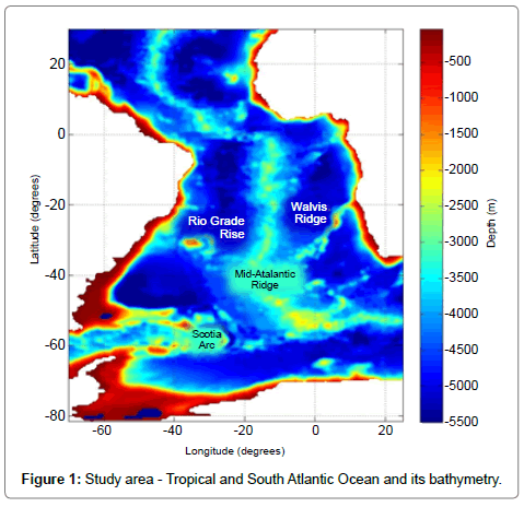
Figure 1: Study area - Tropical and South Atlantic Ocean and its bathymetry.
Pereira et al. [18] observed distributions of chlorophyll-a and net primary productivity (PPL) in the region (from MODIS sensor data), detecting high concentrations in coastal regions, especially near the mouths of great rivers and regions of upwelling or confluence of currents, with marked seasonal variation. That study showed physical variables having high cross-correlation with chlorophyll-a and PPL, but with strong latitudinal dependence and variability in the timing of the biological response, which is greatly influenced by the high seasonality of the physical parameters.
Biological data
Presently, there is a range of sensors coupled to artificial satellites which are used for studies of terrestrial, atmospheric and ocean phenomena. One of these is the Moderate Resolution Imaging Spectroradiometer (MODIS), which is a key instrument coupled to artificial satellites Terra (EOS AM) and Aqua (EOS PM), of the National Aeronautics and Space Administration (NASA). These satellites form a complete coverage of the globe over a period of two days, capturing data in 36 spectral bands at moderate resolution (between 0.25 and 1 km) [19]. Biological data used in this work are horizontal distributions of the concentration of chlorophyll-a based on the lognormal distribution algorithm described by Campbell et al. [20]. These data are derived from remote sensing through MODIS with spatial resolution of 0.5 degrees in latitude and longitude, and temporal resolution of 8 days. Data for the entire period from 2003 to 2009 were used in this study (7 years), with interpolations for missing data due to cloud cover. These data are the product of level 3, provided by Oregon State University (OSU).
The numerical model
The hydrodynamic model used is a version of Princeton Ocean Model (POM) written by Blumberg et al. [21], optimized by Harari et al. [22]. This implementation uses high-resolution grids for the Tropical and South Atlantic and Brazilian Continental Shelf, considering simulations and predictions of circulations generated by tides, winds and density variations. This version has been used for scientific and operational purposes, allowing the reproduction of the hydrodynamics in this area and any subdomain, through nested grids, especially in coastal and continental shelf [22,23].
The POM is a three-dimensional model that considers free surface and solves a set of three-dimensional nonlinear primitive equations of motion, discretized by the finite difference method and considering modes separation. It is through this modes separation that volume transport (external mode) and velocity shear in the vertical (internal modes) are solved separately, saving computation time.
The complete hydrodynamic equations are written in the flux form, considering Boussinesq and hydrostatic approximations. The model also adopts a second order turbulent closure for coefficients of vertical viscosity and diffusion; Smagorinsky parameterization for horizontal viscosity and diffusion; leapfrog scheme for time and horizontal space integration, and an implicit scheme for the vertical integration. For the spatial differentiation, the model uses an alternating Arakawa C-type grid, suitable for high-resolution models (spacing less than 50 km).
The model was processed for 31 years (from 1979 to 2009), the first year being discarded (to avoid the influence of initial conditions at rest). The horizontal grid resolution was set to 0.5° in longitude and latitude, and vertical resolution of 22 sigma (σ) levels of varying thickness, with the first 8 levels corresponding to 10% of the total depth.
The tidal potential was included in all runs and the results of the model were filtered each time step, averaging 5 points in space and 3 levels in time, in order to eliminate noise. The boundary conditions for the currents were fixed as no-gradients and monthly climatological values of temperature and salinity were prescribed at the open limits of the grid. Harmonic constants of tidal components were given at double boundaries, so that the elevations were partially clamped to harmonic oscillations with restoration period equivalent to the baroclinic time step. Table 1 gives some of the conditions used in the model processing and Table 2 informs the input data.
| Model parameters | Values |
|---|---|
| Internal time step (integration) | 1800 s (baroclinic) |
| External time step (integration) | 30 s (barotropic) |
| Coefficient of relaxation to sea surface temperature climatology | 100 W/m2/K |
| Constant horizontal diffusivity (Smagorinsky) | 0,08 |
| Initial value of the Smagorinsky diffusion coefficient | 100 |
| Inverse diffusivity horizontal Prandtl number | 1 |
| Relaxation coefficient of TS model calculations to climatology (for all sigma levels) | 10-3 |
| Weight assigned to the central point in the process of spatial averages | 0,8 |
Table 1: Initial parameters used in the model.
| Input data | Source |
|---|---|
| Bathymetric data | General bathymetric Chart of the Oceans (GEBCO) |
| Forcing of mean sea level at the boundaries is inserted at intervals of 24 h, with corresponding climatological averages. | Ocean Circulation and Climate Advanced Model (OCCAM) |
| Harmonic tidal constants at the open contours | Model TPXO7.1-version utilizes mission data TOPEX / POSEIDON [39] |
| Temperature and salinity annual climatology (inserted at the initial time, at each grid point); | World Ocean Atlas in its 2008 version (WOA08) |
| Relaxation of model results to climatology | Climate Forecast System Reanalysis (CFSR) [40] |
| Boundary conditions for winds and surface fluxes of heat and salt (every 6 hours); | Reanalysis of atmospheric model the NCEP / NCAR [41] |
Table 2: Input data used in the model.
Statistical and spectral analyses
As the outputs of the model were obtained at 6 h intervals, their results were reorganized on 8 days averages, for comparison with the time series of chlorophyll-a, in the same grid points positions of the hydrodynamic model. We applied the method of least squares to obtain trends and annual and semiannual signals of the series [24].
The covariance and cross-correlation functions are used to examine the relationships between different series in the time domain. The mathematical basis for these calculations is provided by Spiegel et al. [25]. By denoting the mean and standard deviation of a time series x as _ x and σ x, and the mean and standard deviation of a time series y as  and
and  both series with N observations, the covariance between series x and y may have time lags h (in this study, h = ..., -2, -1, 0, 1, 2, ... weeks) and is computed as:
And the linear correlation coefficients between series x and y, with lags h, are given by:
The linear correlation coefficient indicates the linear dependence of the compared data, giving the degree of dispersion around an adjustment function that is equivalent to a straight line. The values range between -1 (perfect inverse correlation) and +1 (perfect direct correlation), with values close to zero indicating that the variables in question are not correlated. This parameter estimates then the linear interdependence of two series, where high positive values indicate a similar behavior of the variables, while strong negative values indicate an opposite behavior. For the Fourier analysis of the time series, averages and trends of the series were removed, in order to avoid distortions in the low frequency components of the spectrum [24]. In frequencies domain, the Fourier transform of a time series is defined as:
where  and
and  are defined based on the observation period T:
: 
Finally, the cross-spectrum is defined by the Fourier transform of the cross-covariance function (6) whose amplitude peaks indicate the frequencies where there is a greater inter-relationship between series and phases indicate their respective delays (in time).
Distribution of chlorophyll-a
The distribution of the mean values of chlorophyll-a (Figure 2a) showed behavior similar to that observed for long-term analysis with remote sensing data held by Deser et al. [26], Hardman et al. [27] and Saraceno et al. [28], and optimal interpolation observational data by Reynolds et al. [29] For all the study area, this distribution had a mean of 0.31 ± 0.78 mg/m3. One can observe a pattern of high concentrations in regions of coastal upwelling, equatorial upwelling and high latitudes. These results corroborate those obtained by Wang et al. [30] for the climatology of SeaWiFS data in the period 1997-2007, which also checks the seasonality of chlorophyll-a in the equatorial region, the Amazon and Congo River discharge areas and upwelling regions in North Africa, as can be observed in the distribution of the standard deviation of the annual and semiannual signals.
The distribution of the chlorophyll trend (Figure 2b) showed an average of (0.22 ± 3.79).10-2 mg/m3/year. The largest variabilities (both positive and negative) concentrated in the coastal regions, with the highlight of a region with negative trend near the mouth of the La Plata River.
The distribution of the standard deviation (after removal of annual and semiannual signal) had a mean of 0.22 ± 0.75 mg/m3 (Figure 2c). This distribution pattern is similar to that of the mean concentrations, with higher standard deviation in the regions of higher mean concentration. The spatial distribution of the standard deviation of annual and semiannual signals averaged 0.03 ± 0.10 mg/m3 (Figure 2d), with values much lower than those found in the residual signals, indicating that although the seasonality is important, it does not represent the largest part of the chlorophyll variability. Garcia et al. [31], by means of spectral analysis, found and highlighted the significance of the signal in the annual and semi-annual variability of chlorophyll-a in the region of the Malvinas Current, with similar values to those of the residual distribution, but their signals were more evident in the region north of the belt of 40°S. Hardman et al. [27] verified the high values of overall standard deviation in the Congo River Plume, probably contaminated by high loadings of suspended particulate matter and dissolved organic substances and strong biannual signature.
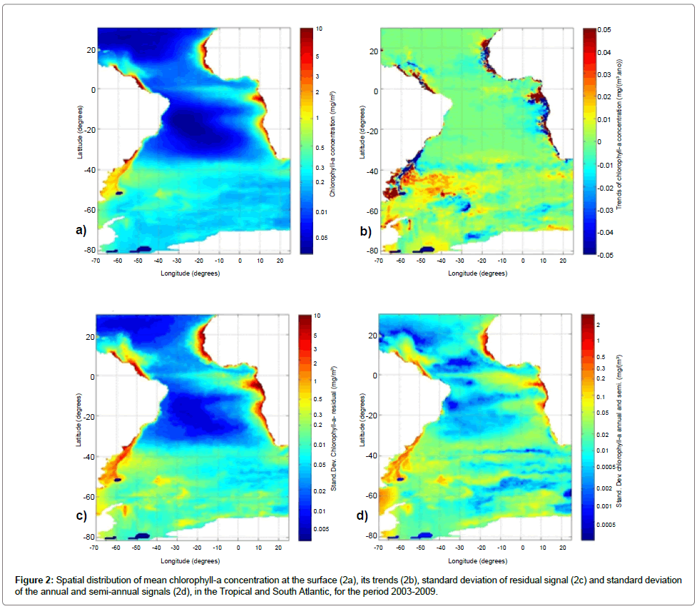
Figure 2:Spatial distribution of mean chlorophyll-a concentration at the surface (2a), its trends (2b), standard deviation of residual signal (2c) and standard deviation of the annual and semi-annual signals (2d), in the Tropical and South Atlantic, for the period 2003-2009.
Correlations between chlorophyll-a and physical variables
Distributions of the linear correlation coefficients between chlorophyll-a and the physical variables computed by the model, considering zero time lag, are shown in Figure 3, for the Tropical and South Atlantic. The distribution of the correlation coefficient (with zero lag) between the current intensity and chlorophyll-a (Figure 3a) has average of 0.00 ± 0.08, with a maximum of 0.38 and minimum of -0.41, with no defined pattern. Anyway, it is possible to detect a belt of positive correlations in the equatorial region and a point of negative correlation near the mouth of the Amazon River.
The correlation between the surface elevation and chlorophyll (Figure 3b) has an average of -0.02 ± 0.13, with maximum of 0.37 and minimum of -0.48. Despite having values comparable to those found in the correlation with the intensity of the currents, this distribution showed a more defined spatial pattern, so that in the area of the triangle of positive elevation (SASG) predominates negative correlation coefficients. The equatorial region, south of the North Atlantic Subtropical Gyre (NASG) and a belt around 45°S also display negative correlations. For salinity, the correlations with chlorophyll-a averaged -0.02 ± 0.12, with maximum and minimum of 0.44 and -0.58, respectively (Figure 3c). This distribution showed no defined spatial pattern, but is characterized by the predominance of positive correlations at high latitudes (up to latitude 40°S) and a belt between the Equator and 10°N. The region of the mouth of the Amazon River showed negative correlations. This fact would suggest that the lower salinity site (the larger river discharge), the greater supply of limiting nutrients in the process of photosynthesis. And for temperature, is seen spatial average of 0.02 ± 0.17, with a maximum value of 0.68 and a minimum of -0.57, shown in Figure 3d, with a well-defined distribution pattern, having positive values at high latitudes (up to 40°S), and a region with negative values constrained by Brazil Malvinas Confluence (BMC), the South Atlantic Current (SAC) and the Agulhas Current Retroflection (ACR). A high positive correlation in the region of the Amazon and Congo River discharges and in the region near to the northeastern coast of Brazil can also be observed. Picaut et al. [32] presents a pattern of distribution for this seasonal signal of sea surface temperature in the Atlantic equatorial region similar to that shown by the chlorophyll-a (Figure 2d), which justify this high and almost homogenous negative correlation in this region. In medium and low latitudes, the temperature rise drives a stepping thermocline, forming a thermal barrier that hinders the entry of nutrients from the deeper layers into the mixed layer. Thus, there is a reduction of primary productivity. On the other hand, at high latitudes, the low temperatures prevent the formation of a thermocline, so that the temperature rise is indicative of solar radiation increase, resulting a deeper penetration of radiation into the water column, resulting then a primary productivity increase.
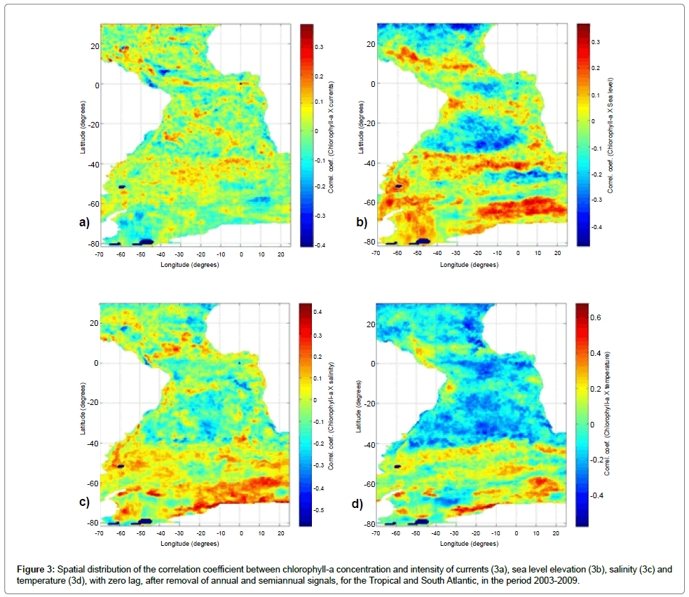
Figure 3: Spatial distribution of the correlation coefficient between chlorophyll-a concentration and intensity of currents ( 3a), sea level elevation ( 3b), salinity ( 3c) and temperature (3d), with zero lag, after removal of annual and semiannual signals, for the Tropical and South Atlantic, in the period 2003-2009.
Next, Figure 4 presents the distributions of maximum crosscorrelations between chlorophyll-a and physical variables considering the respective time lags. Negative lags mean advance of the physical variable with respect to the biological one, while positive lags mean delays in the occurrence of the physical variables. The time unit in the considered lags is equal to 8 days (approximately one week). The distribution of the cross-correlation with the intensity of currents averaged 0.01 ± 0.15, with extremes of 0.41 and -0.41 (Figures 4a and 4b). Note a slight change in the distribution of these correlations relative to zero lag, like a band of positive correlations in the equatorial region, with negative lag of up to 10 weeks, which means the physical variable precedence in relation to the biological variable. There are regions of negative correlation, like near the mouth of the Amazon River, but there are regions with positive correlations, as in the southern and southeastern Brazilian coast, lagged positive in approximately five weeks. This positive correlation at the equator is plausible when considering the increased intensity of the currents in the region as a result of increased intensity of trade winds, since this system is responsible for upwelling in the region, due to the winds and consequent Ekman transport mechanism, which generates currents with southern components. The greater intensity of winds the greater intensity of the currents, and the greater intensity of meridional currents. This would generate a greater vertical transport in the area, increasing the supply of nutrients from deeper layers into the surface. The occurrence of high correlation values in module, with both positive and negative lags, highlights the existence of a factor that influences the variability of both variables correlated, with no necessarily cause and effect relationship between these variables. The cross-correlations between chlorophyll-a and sea level elevation showed a mean value of -0.02 ± 0.20, with maximum and minimum of 0.51 and -0.48, respectively (Figures 4c and 4d). Can be noted, in this distribution, a reinforcement of what was found previously with zero lag. The triangle elevation keeps negative correlation, with virtually zero lag, this behavior followed in equatorial regions and NASG. In regions of positive correlation there is predominance of positive lag, but with much variability. A strong negative correlation in the region inside the SASG may suggest that the increase in surface elevation causes an increase in the thermocline depth, removing the region below this layer (more nutrients) in the photic zone, which would reduce the primary productivity. This type of event would have a biological response almost immediately.
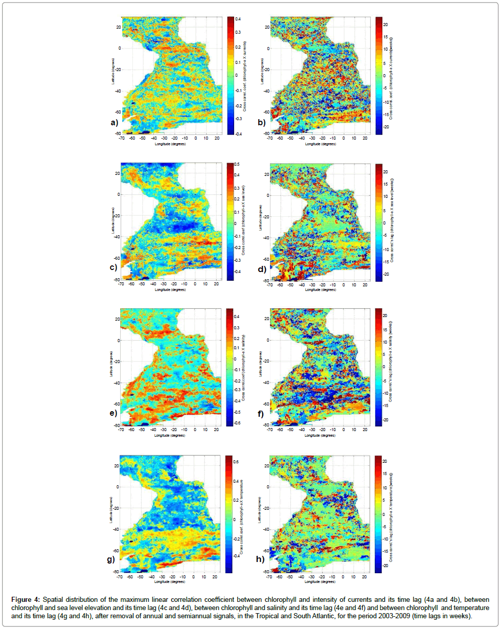
Figure 4: Spatial distribution of the maximum linear correlation coefficient between chlorophyll and intensity of currents and its time lag (4a and 4b), between chlorophyll and sea level elevation and its time lag (4c and 4d), between chlorophyll and salinity and its time lag (4e and 4f) and between chlorophyll and temperature and its time lag (4g and 4h), after removal of annual and semiannual signals, in the Tropical and South Atlantic, for the period 2003-2009 (time lags in weeks).
With salinity, the cross-correlations averaged -0.04 ± 0.21, with maximum and minimum values of 0.48 and -0.64, respectively (Figures 4e and 4f). In this distribution there are similarities with the distribution of the simple zero lag correlation, with a predominance of positive correlations at high latitudes and a belt above the equator, these ones being associated with negative lags of more than 15 weeks. The negative correlations, especially the most intense in the region near the Antarctic continent, are associated, in general, to positive lags.
The same correlation with temperature showed a mean value of -0.02 ± 0.22, with 0.68 maximum and -0.57 minimum (Figures 4g and 4h). This distribution confirms the pattern already seen in the simple zero lag correlation, highlighting the association of this correlation to a virtually instantaneous response time.
Analysis of transect 20°W
Next, latitudinal variabilities at the longitude of 20°W of the amplitudes of the Fourier spectrum of the cross-covariance and respective time lags (in years), between chlorophyll-a and physical variables, are presented on Figure 5. For the intensity of currents and surface elevation there are greater amplitude for low frequency signals (more than 3 years) with great variability in response time, oscillating positive and negative values over 1 year. These signals are concentrated in the belts of 10°N to 30°N, between 30°S and 40°S and around 60°S to 70°S, concentrating on the period of 7 years (equivalent to the extension of the series). Peaks in the spectrum with periods of 6 and 7.5 years have been cited in the analysis of IOS and ION [32], which emphasizes the shortness of the series analyzed. There is a weak signal in the period of 2.3 years, with response almost instantaneous (lag zero) most salient between the Equator and 10°S. For surface elevation, across the transect is evident a strong signal with period of 0.33 years and a less intense one located between 35°S and 60°S of 0.25 years (Figures 5c and 5d). Alvarez- Ramirez et al. [33] associate the signal of period 0.33 years with the frequency spectrum of the Northern Oscillation Index (NOI), related to the North Atlantic Oscillation (NAO), with nonlinear resonant effects. The period of 0.25 years, as it is a submultiple of the annual signal, can also be related to a resonant effect associated with seasonality. There is also a weak signal in the period of 1.4 years (at approximately 15°S) and 1.7 years (at approximately 35°S) with response almost instantaneous.The transects for salinity and temperature amplitudes present the most striking features for certain frequencies, with evident signatures at low frequencies (Figures 5e and 5h). Lags have similar patterns to those found for other physical variables (with more immediate responses to higher frequencies), but with regions of alternating signals better defined. These low-frequency signals are concentrated in the period of 7 years (extension of the time series itself). These transects, as well as surface elevation, clearly feature the signal of period 0.33 years in much of the transect, intensified in the polar region. At high latitudes, similar to the other physical parameters, salinity and temperature have highlighted signals of lower frequencies (period 2.3 years) concentrated from 30°S to 40°S and between the Equator and 10°S, both with positive lag about 1 year. Mainly for high latitudes, there are signals with periods around 1 year which can be due to failure when removing the seasonality. It is also apparent, particularly in the region between 10°N and 20°N, a signal with period of approximately 1.4 years, with a positive phase shift below 6 months. Note that this region is affected by coastal upwelling (North African coast).
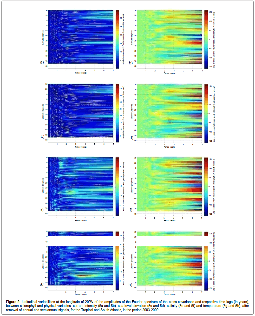
Figure 5: Latitudinal variabilities at the longitude of 20°W of the amplitudes of the Fourier spectrum of the cross-covariance and respective time lags (in years), between chlorophyll and physical variables: current intensity (5a and 5b), sea level elevation (5c and 5d), salinity (5e and 5f) and temperature (5g and 5h), after removal of annual and semiannual signals, for the Tropical and South Atlantic, in the period 2003-2009.
For temperature, greater emphasis is given to the occurrence of a signal with high amplitude in the belt between 50°S and 60°S, also present but weaker in 5°N, with higher values around 3.5 years and having a negative gap of less than 6 months. There is also the occurrence of weaker signals concentrated around the period of 2.3 years, at 10°N and 45°S with an almost immediate response (delay less than 10 weeks). The occurrence of these same signals is verified for salinity, but with greater intensiy in the period of 2.3 years, concentrated between the Equator and 5°S and around 45°S (region of higher salinity gradient).
Carton et al. [34] highlights variabilities in the equatorial mode of the sea surface temperature for a timescale of 2-5 years like being controlled by dynamical processes. Hardman-Mountford et al. [27] observed cycles with periods between 3 and 5 years in spectral analysis of time series of surface temperature anomaly and wind components for the equatorial region, north of Angola and Benguela, in the period from 1982 to 1999. The same period is highlighted in the analysis of wavelet transform (disregarding the annual signal) in 32-years integration of ROMS (Regional Ocean Modeling System) for the same region by Colberg et al., [35], with the variability related to coastal Kelvin waves associated to ENSO events in the Tropical Pacific.
Schneider et al. [32] found that the variance spectrum of the Southern Oscillation Index (SOI) showed significant peaks with periods of 2.3, 2.9, 3.5 and 6 years. Phenomena of El Niño - Southern Oscillation (ENSO) show interannual components ranging between 2.3 and 3.4 years and a low frequency component of 6 years or more, being the period of 2.3 years consistent with the average periodicity of ENSO [36]. Thus, we can associate the signals of periods 3.5 and 2.3 years to ENSO phenomena. This periodicity is verified for Naujokat et al. [37] that found a quasi-biennial oscillation with mean period of 27.7 months (2.308 years) in equatorial zonal winds data that can suggest the ocean atmosphere coupling. Other signals are observed with low intensity, as for the period of 1.7 years evident at 35°S, with negative delay of about 6 months to temperature, and the period of 0.7 years and instantaneous response, concentrated at high latitudes in temperature and salinity, but prominently in temperature. The signature of period 0.7 years closely resembles that analyzed for 0.33 years. Schneider et al. [27] found that the variance spectrum of the NOI had significant peaks at periods of 1.7, 2.2 and 7.5 years, which allows to associate this signal of 1.7 years with the analyzed signal in NOI. In analyzing the Magnitude of the Squared Coherence for temperature anomalies of the sea surface and the SOI, Campos et al. [38] found spectral peaks of frequencies 0.12 and 0.055 cycles per month (equivalent to the periods of 0.7 and 1.5 years, respectively), relating them to the ENSO phenomena.
The distributions of mean values and standard deviations of chlorophyll-a exhibit behavior similar to that given in literature. The annual and semi-annual signals are predominant both in MODIS and model data but, even excluding these components; the residual correlations are still high. On the other hand, annual and semi-annual signals have smaller standard deviation than the remaining (residual) frequencies. The cross-correlations between chlorophyll-a and salinity, temperature and surface elevation showed spatial distribution patterns with well defined latitudinal character, presenting higher modulus of correlation for temperature and salinity, above +0.6 in the polar region and below -0.5 in the tropical area. A general pattern of negative correlations in the regions of low concentration and positive in regions of high concentration was obtained, except the Equator (region of high chlorophyll-a concentration, which is characterized by a negative correlation for all variables, except the intensity of the currents). The cross-correlations between chlorophyll-a and physical parameters corroborate the pattern found in the correlations considering lag zero, stressing aspects as the positive correlation with the intensity of the currents in the equatorial region and the negative correlation with the surface elevation inside the SASG, both presenting immediate response. In the analysis of spectral distributions of Fourier spectra of the cross-covariance between chlorophyll-a and each of the physical variables, in the transect 20°W, the best defined signals were found for temperature and salinity, especially the periods of 3.5, 2.3, 0.7, and 1.7 years, with varying spatial distribution and time lags. These signals are found in the literature, being associated with ENSO phenomena. Thus, one can conclude from this study that there is a very characteristic spatial distribution of correlations between physical variables and chlorophyll-a, even removing the annual and semiannual signals. Despite their importance, these signals are not responsible for much of the variability of chlorophyll-a concentrations. It should be noted also that the spatial variability also occurs in the frequency domain, which denotes a probable influence of ENOS phenomena, both in the physical variables and chlorophyll-a. As a suggestion for future work, further research should focus on the causes of the spatial variability of the correlations and phase delays, as well as a better understanding of how phenomena such as ENSO (El Niño - Southern Oscillation) affect these correlations.