Journal of Geology & Geophysics
Open Access
ISSN: 2381-8719
ISSN: 2381-8719
Research Article - (2012) Volume 1, Issue 1
Six iSPHERE oil spill and current tracking buoys were deployed over the continental shelf of northern Norway (Nordkapp region) during spring-summer 2011. These drifters provide real-time GPS position location information to aid in locating marine oil spills and other leeward drifting objects. In this study we assess the differences between the spreading of the surface drifters and the trajectories forecast by the operational Lagrangian oil drift model at the Norwegian Meteorological Institute (met.no). The study investigates the reason for these differences, and we use a recently established new skill score as a measure of the model accuracy. The differences observed in this study are the consequence of the combined impact of the modeled wind, ocean and current constituents that force the oil drift model. Each numerical model is run on a grid of 4 km resolution, which means that many mesoscale features are either not represented well enough, or not represented at all. A problem with the ocean model, since eddies in the ocean are typically of a much smaller scale than in the atmosphere (40-50 km), and there are few observations to assimilate into the model. Studies such as this, comparing modeled trajectories with observed drifter trajectories are an important way to indirectly validate and improve ocean models, as well as improving the trajectory model itself.
Keywords: Oil-spill model, Comparison of trajectories, Trajectory model, Model assessment, Oil-spill model assessment
Lagrangian drifter measurement programs can be divided into studies of surface currents and of sub-surface currents. There are more than 1200 drifters in all ocean basins as part of the World Drifter Program (www.aoml.noaa.gov). The drifters typically include a satellite-tracked transmitter and frequently an under surface drogue. Lagrangian statistics concern averages of particle positions, velocities are related quantities over many realizations. The measurements can be separated into those pertaining to single particles and those requiring two or more particles. Both single and multiple particle statistics are required for a full description of tracer evolution [1].
During our research cruise we deployed surface drifters. The iSPHERE is an expendable, low cost, bi-directional spherical drifting buoy. The buoy was designed specially to track and monitor oil spill incidences. The iSPHERE drifter also provides the user GPS positional data. This buoy responds to the atmospheric forcing, surface waves and the ocean circulation, with various degrees of coupling between the systems.
In this paper we use a method based on the Lagrangian separation distance between the endpoints of simulated and observed drifter trajectories to assess the performance of the oil drift model. We have a restricted quantity of drifter observations that extend over both coastal zones and continental shelf areas. As is well known, Lagrangian assessments are for the most part based on drifter trajectories and their Lagrangian statistics [2]. Following McClean et al. [3] we compared the time and length scales of dispersion based on Lagrangian autocorrelation functions [4].
Lagrangian velocity statistics, calculated over large group of particles, correspondingly need a large number of drifter paths. Recently, Ohlmann and Mitarai [5] performed a purely Lagrangian validation of surface current dispersion simulations in the coastal ocean and simulations based on Lagrangian probability distribution functions (PDFs) [6,7]. The interaction between the Lagrangian PDFs for current and simulated drifters is determined using the Kolmogorov – Smirnov (K-S) statistical test [8-10], which assumes a maximum diversity in the cumulative distribution functions.
The trajectories provide information about both the paths and structures of the sampled characteristics. Drifters and floats have also been used to deduce the structure of large-scale currents like the Gulf Stream.
Nevertheless, the ocean is extremely changeable, both spatially and temporally. The particles deployed at the same location with little separation in time may sometimes follow similar paths, yet at times are separated in completely different paths. Thus, it is not reasonable to talk about the path of a single drifter, since that path is almost surely unequalled. As acknowledged previously by turbulence researchers, such indeterminacy necessitates a statistical or probabilistic explanation, deduced from complexes of trajectories.
In our research we have looked closely at the different weather conditions during our observations because it could be one of the main reasons of possible errors. Through this analysis we have established some means of improving our oil drift model.
Close to our region of research, the Goliat oil field was discovered in 2000 – one of the most recent major oil finds (Figure 1). It has two main formations (Kobbe and Realgrunnen) and two minor formations (Snadd and Klappmyss) with recoverable reserves of 174 million barrels (27.7×10⁶ m3) (www.offshore-technology.com). The proximity of the Goliat oil field to an area of significant biological productivity highlights the importance of having an operational system for the precise tracking of oil spills. When an oil spill occurs at sea, the first and greatest concern of response planners is to determine where the oil is likely to go. Tracking oil spills is of prime importance for effective planning and deployment of oil spill response personnel and equipment to protect environmentally sensitive areas.
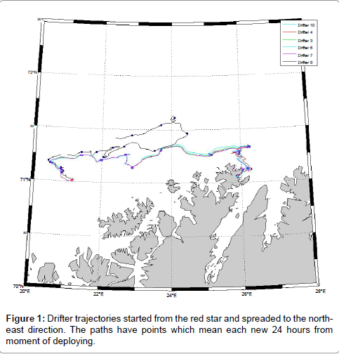
Figure 1: Drifter trajectories started from the red star and spreaded to the northeast direction. The paths have points which mean each new 24 hours from moment of deploying.
The region of deployment is located north of Norway and remains ice-free year round due to the warm Nordkapp current. The thermohaline circulation affects the climate in the area, and the regional climate can deviate significantly from average.
The thermal convection between the relatively warm water and cold air in the winter plays an important role in the region. The 10-degree July isotherm runs through the region and is often taken as the southern boundary of the Arctic. The region generally has the lowest air pressure in winter. The water temperature is 3-5°C in February and 5-8°C in August [11].
There are two main types of water masses: warm, saline Atlantic water (temperature >3°C, salinity >35‰) and warm, but not very saline coastal water (temperature >3°C, salinity <34.7‰). The hydrology of the upper water layers is largely determined by the flow from the North Atlantic and form eddies in an anti-clockwise motion. A portion of warm surface water flows north along the Norwegian coast from the Norwegian Sea forming the Nordkapp current with a speed of 0.9–1.8 m/s and a volume transport of 1 Sv (1million m3/s). This water is cool enough to submerge into the deeper layers; there it displaces water that flows into the North Atlantic.The tides have a semi-diurnal character with currents of floods and ebbs, its amount to 4.7 m [12].
Due to the North Atlantic drift, the region has a high biological production compared to other oceans of similar latitude. The spring bloom of phytoplankton can start quite early. The phytoplankton blooms feeds zooplankton. The zooplankton feeders include young cod, capelin, polar cod and whales. The high biological productivity makes this a region of high ecological importance.
In this article we will focus on possibilities for tracking oil spills on the surface using met.no’s OD3D model system, analyzing its strengths and weaknesses.
For our studies we used the Lagrangian autocorrelation and dispersion indicators and a new skill score for evaluating trajectory model performance. Here, we examine the statistical indicators of our model.
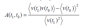
The autocorrelation function of a Lagrangian velocity component v can be defined, for t1 ≥ t0 as:
 (1)
(1)
In our case, the autocorrelation function depends on the time lag t = t1-t0. Here our autocorrelation function will be close to zero in context about the integral Lagrangian time.
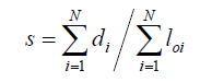
Further presented is the new skill score for data from the research cruise. According to Liu and Weisberg [2], a Lagrangian trajectorybased non-dimensional function can be determined as:
 (2)
(2)
where di is the separation distance between the end points of observed and simulated trajectories at the time segment l after the start point (virtual particle release), loi is length of the drifter’s trajectory, and N is the number of time segments (Figure 2). The smaller the normalized cumulative separation distance (s), the better the model simulation compares with the real observations. s = 0 would be a perfect match between observed and simulated trajectories.

Figure 2: Visualization of determination of parameterizes for determination of the normalized cumulative separation distance, where lo and lm are the lengths observed and modeled paths, respectively.
s = (d1 + d2 + d3) / (l01 + l02 + l03)
where:
l01 = dl1
l02 = dl1 + dl2
l02 = dl1 + dl2 + dl3
The idea of this function is to normalize the Lagrangian separation distance di between the modeled and observed drifter path with the length of the path loi. Based on s we can calculate the skill score ss for s<0.5:
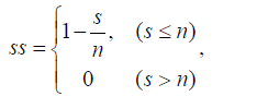 (3)
(3)
where n is a non-dimensional, positive value that determines the limit of no skill (ss = 0). In the case of s = 1 we have for ss:
 (4)
(4)
Here model simulations uses s > 1 are flagged to be no skill (ss = 0). This corresponds to the condition that the cumulative separation distance cannot be larger than the associated cumulative length of the drifter path, i.e.,
and we can say, that in this case, the model has no skill. Here the skill score (ss) is in the range of 0 (no skill) to 1 (ideal modeling). As discussed in Liu and Weisberg [2], this dimension less skill score is particularly useful in model evaluation when the number of drifter trajectories is limited.
Comparison of weather components
The following hours; 0, 122 and 216 were chosen deliberately. At these times our model and the observations were almost completely uncorrelated and spread in different directions and at different speeds (Figures 3-5). Under the influence of certain weather conditions the drifters would follow one path and the model particles would follow a very different one. The weather conditions at the three chosen time steps are described in the table (Table 1).
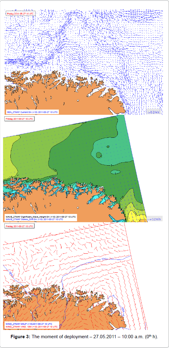
Figure 3: The moment of deployment – 27.05.2011 – 10:00 a.m. (0th h).
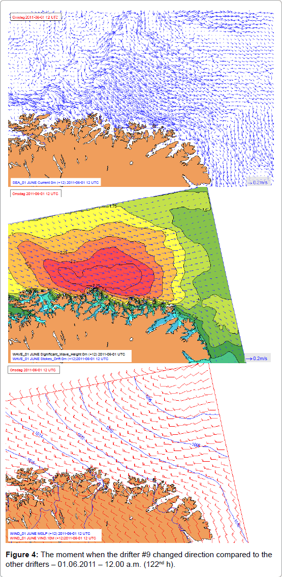
Figure 4: The moment when the drifter #9 changed direction compared to the other drifters – 01.06.2011 – 12.00 a.m. (122nd h).
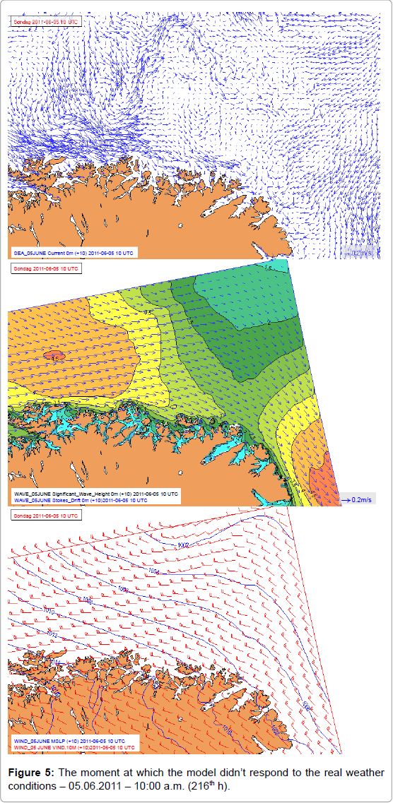
Figure 5: The moment at which the model didn’t respond to the real weather conditions – 05.06.2011 – 10:00 a.m. (216th h).
| Hour\Components | Current | Wave | Atmospheric |
| 0th Fig.3 | 130º, 0.2m/s | 80º, 1.2m | 40º, 2.5m/s, 1012 hPa (hpz1) |
| 122nd Fig.4 | 110º, 0.3-0.4m/s | 85º, 0.2m | 85º, 7m/s, 1011 hPa (hpz1) |
| 216th Fig.5 | -º *, 0.1m/s | 100º, 0.1m | 90º, 5m/s, 1007 hPa (hpz1) |
Table 1: Weather data extracted from the met.no models.
To compare the various weather components we extracted our data from different models (atmosphere, ocean and wave).
Current components: Ocean currents at several depths as well as temperature and salinity were supplied by the met.no version of the Princeton Ocean Model, which is a regional model with 4 km horizontal resolution.
Wave components: The local wave field is given by the wave model WAM with 4 km resolution. The Stokes drift computed by WAM is used to advect the oil in addition to the contribution of wind and currents. The Stokes drift (Stokes, 1847) is an integrated measure of wave momentum in frequency and direction space. Significant wave height and mean period are used to calculate turbulent diffusivity and dispersion.
Atmospheric components: Wind at 10 m above the surface is taken from the atmosphere model HIRLARM (High Resolution Local Area Modeling) with 4 km horizontal resolution. This is the operational weather forecasting model at met.no.
Drifter measuring
The data collection took place in the small area at the interface between the Norwegian and Barents Seas May 27 – June 09 in 2011. Drifters (iSPHERE from MetOcean) were deployed at 71.0°N, 21.2°E and spread towards the north-east (Figure 1).
These drifters follow the surface currents and are also affected by wind. They are designed specifically so that wind and currents will influence their movement, simulating the behavior of an oil spill on the sea surface.
The iSPHEREs are spheric floats with a diameter of 39.5 cm and a mass of 10.9 kg. They are half submerged in the water and therefore exposed to the wind. They have an aerodynamically smooth shape and previous studies indicate that this type of float drifters in a manner similar to the behavior of crude oil (Aamo and Jensen 1997 [13]). Their main use is for oil spill tracking.
The drifters transmit their positions over the Iridium satellite network. The positions are reported every 30 minutes. The iSPHERE investigation started at 10:00, 27.05.2011, deploying the drifters at the same time with only slight position differences. The collection of data was stopped at 23:30, 09.06.2011.
Simulation
The Oil Drift 3-Dimensional numerical model system (OD3D) at Met.no was designed in cooperation with SINTEF and based on superparticles which depend on the atmosphere, ocean and wave (containing the Stokes drift) field. All of them can be extracted from the weather models described above. The OD3D contains parameterizations of the main processes that influence the oil, such as horizontal dispersion, mixing within the water column, oil weathering and others.
In our experiment the OD3D model time step is 15 minutes. The model can predict the spreading, evaporation, mixing, dispersion, submerging and beaching during a simulation.
In the operational setup, OD3D extracts data from the Nordic 4 km and Skagerrak 1.5 km, but the oil drift model can be launched using various atmospheric, wave and ocean models in a non-operational mode [14].
The model resolution was too coarse to resolve some eddies during the experimental period – and other eddies were not simulated correctly in time and space. This resulted in a straight modeled trajectory at a time when the observed drifter got caught in an eddy and went off on a completely different track. We can see some of the different tracks in Figure 1.
A comparison of the velocities of observed and modeled particles is shown in Figure 6. Here it is clear that the velocities of observations have more variability and high amplitudes due to the tidal signal. The modeled mass center speed in an average over 500 particles spreading in different directions.
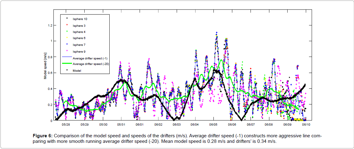
Figure 6: Comparison of the model speed and speeds of the drifters (m/s). Average drifter speed (-1) constructs more aggressive line comparing with more smooth running average drifter speed (-20). Mean model speed is 0.28 m/s and drifters’ is 0.34 m/s.
Average drifter speed (-1) and average drifter speed (-20) are running averages with different time steps +/-1 and +/-20, respectively. The running averages of the drifter speeds contain tidal effects, and so the drifter speed lines fluctuate with a higher frequency than the model speed line. This is particularly clear in the +/-1 average, while in the +/- 20 average the tidal effects are smoothed out more.
In addition to comparing the speeds, the velocity was broken down into u and v components and these were compared for model and observations (Figure 7). The observed u and v components show more static motions compared with the modeled.
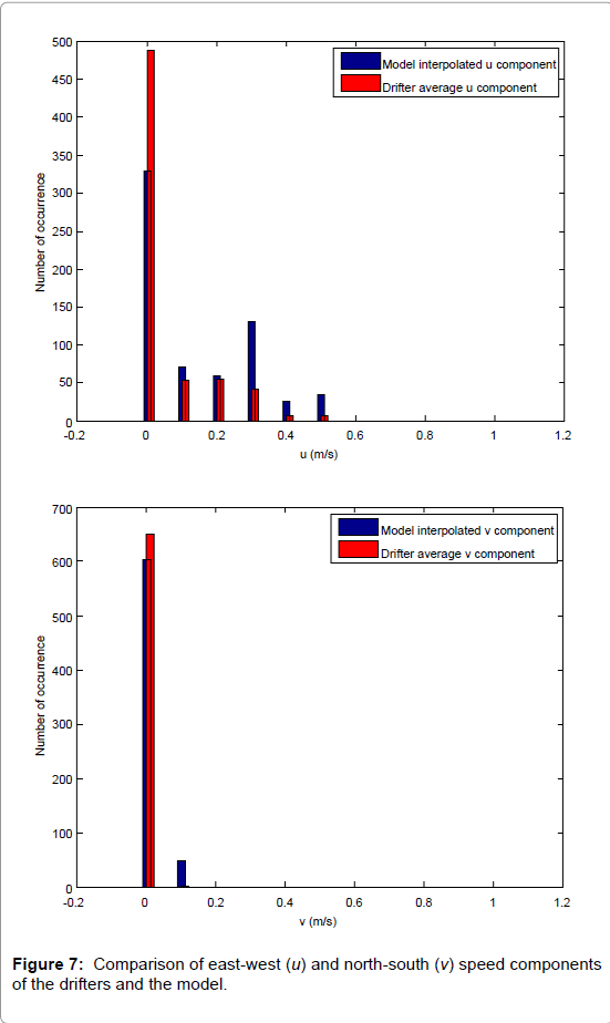
Figure 7: Comparison of east-west (u) and north-south (v) speed components of the drifters and the model.
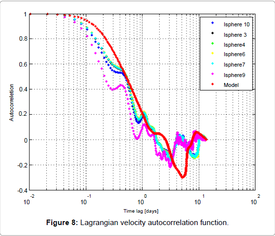
Figure 8: Lagrangian velocity autocorrelation function.
Finally, Figure 9 shows the trajectories of the drifters and model. Here it is clear that the initial point of separation took place right away after the start of our experiment. Calculations showed that each drifter travelled on average almost 67 km. The trajectory of the model is almost the same length, but with a lower average speed (Figure 6).
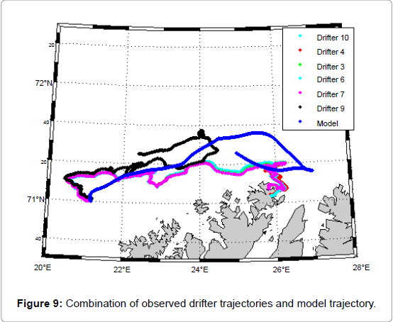
Figure 9: Combination of observed drifter trajectories and model trajectory
This again indicates that the drifters were involved in some horizontal mixing due to eddies. This mixing played an important role in the drifters’ separation. The latter led to the beaching of a separate group of drifters. Another drifter (#9) got caught up in eddies or meanders, which are not consistently reproduced in the ocean models, and the drifter went in a northerly direction.
Using (2), the calculation shows that the Lagrangian separation distance is equal to 0.2698.
Here we have presented two calculated skill scores for the model with different classes of reliability by putting n = 1and then n = 0.5 in (3) and (4), but ss(0.5) dips below the zero line, which means that the model has no skill. This implies that ss(1) is more useful with a value equal to 0.7302. The resultant skill score and normalized cumulative separation distance are shown in Figures 10 and 11. At 27.05-30.05 the model performs comparatively worse (the s increases during 27.05.2011-02.06.2011) missed by input data as it were shown on the weather conditions (Figures 3-5). But after this the simulation improved (31.05-04.06) and the summary error and separation distance decreased by almost 59% and 76%, respectively (04-09.06).
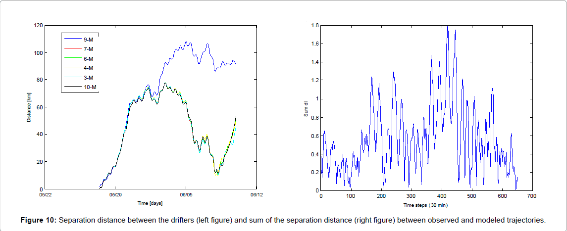
Figure 10: Separation distance between the drifters (left figure) and sum of the separation distance (right figure) between observed and modeled trajectories.
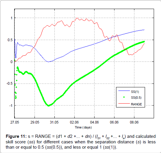
Figure 11: s = RANGE = (d1 + d2 +... + dn) / (l01 + l02 +... + ln) and calculated skill score (ss) for different cases when the separation distance (s) is less than or equal to 0.5 (ss(0.5)), and less or equal 1 (ss(1)).
Forecasting of oil spill spread and drift is very complex and includes several processes. Observations were compared with simulated locations and speed components. There are several reasons for the observed discrepancy, but first of all it is a geographical region with a highly energetic ocean zone with a strong thermal gradient and great variability, where the Arctic and Atlantic oceans are connected. It means a lot of mesoscale structures that are not resolved by the ocean model.
We have shown the particle analysis by calculating values such as the Lagrangian autocorrelation function. The skill score, based on the cumulative Lagrangian separation distance standardized by the associated cumulative trajectory length, proved to be a useful parameter to evaluate the model performance, rather than just using a separate day validations. We calculated it for the estimation of surface trajectories calculated by OD3D for the Nordkapp region in 2011.
Studies (e.g. Forget and André [15]) indicate that chlorophyll imagery can be used as a tracer of surface dynamics, albeit with limitations, especially near the coast. The chlorophyll concentration in (Figure 12) can be seen as illustrating the dynamics of the sea surface waters. Eddies are usually associated with high biological activity, and so the area of high chlorophyll concentration could indicate the presence of an eddy. Our hypothesis is that drifter #9 has drifted along the front between the two water masses and got caught up in an eddy transporting it northeastwards, while the other drifters have followed the waters flowing in an east-southeast direction. This is supported by data from the ocean model, which shows a high variability in the surface waters in this region at the same period.
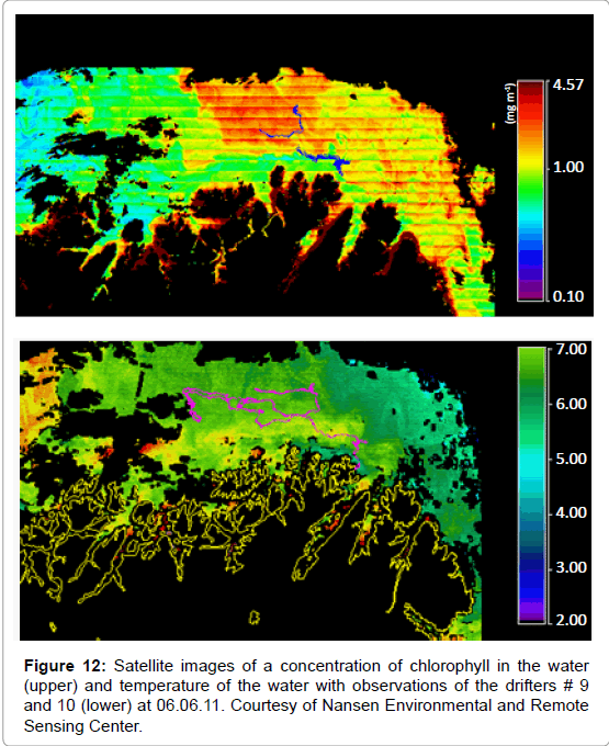
Figure 12: Satellite images of a concentration of chlorophyll in the water (upper) and temperature of the water with observations of the drifters # 9 and 10 (lower) at 06.06.11. Courtesy of Nansen Environmental and Remote Sensing Center.
The results of our experiments lead us to the following conclusions:
1. Location and speed errors in the start of the simulation are one of the main reasons for the divergence between model and observations, and these errors will increase with time.
2. In general, operational oil spill models perform better during first 2-3 days. In our case, the model performed better from 3-4 days after the start of the experiment and showed improvement until day 13. The drifters were deployed in a coastal ocean where the currents are steered by the bathymetry and coastlines, and the separation distances between the modeled and observed trajectories tend to be reduced accordingly (due to lack of velocity component in the across-shore direction). In a normal mode, operational oil spill trajectory forecasts should be frequently re-initialized to reduce the forecast errors which may be accumulated from the initial locations (conditions), as learned from the rapid response to the Deepwater Horizon oil spill in the Gulf of Mexico (e.g., Liu and Weisburg [2]).
3. The main reasons for possible errors are features such as eddies, inertial oscillations, tides and so on, which have local occurrences and are difficult to forecast.
4. An increase of model sensitivity in 4 km resolution will make it possible to use it more efficiently on different times (e.g. 1-4 days).
5. The model needs more observations to improve wind-wave-currentforcing functions that are used to drive the model. A higher number of drifters (30-50 for the observed region – as opposed to the ocean region where it would be more efficient to deploy for example 1000 drifters) is necessary to provide for model validation.
A new operational ocean model with 800 m horizontal resolution is about to be set up at met.no. It is based on the Regional Ocean Model System (ROMS). New comparisons with different drifter trajectories will be carried out with the new model setup.
We would like to thank Ole Johan Aarnes of Norwegian Meteorological Institute for help in the technical development and unstinting support and Annette Samuelsen of Nansen Environmental and Remote Sensing Center for given satellite images and two anonymous reviewers for detailed comments on the manuscript. This research was supported by the BarentsWatch program and the Research Council of Norway (RCN) through the project BioWave (havKyst program) and BarStat (Yggdrasil program). This research was made possible in part by a grant from BP/The Gulf of Mexico Research Initiative.