Journal of Proteomics & Bioinformatics
Open Access
ISSN: 0974-276X
ISSN: 0974-276X
Research Article - (2017) Volume 10, Issue 11
Mtr homology model requires structural refinement to erroneous regions that are not aligned correctly to the template. In this study, refinement methods: LM, MDS, 3Drefine, GalaxyRefine and FG-MD were compared. Errat plot showed a gradual increase in the overall quality factor of ~96% using LM, while there was abrupt increment of >90% for MDS, GalaxyRefine and FG-MD. In the case of LM, structure compatibility decreased to ~53%, whereas it increased to >74% in case of MDS and GalaxyRefine. Ramachandran plot showed residues in favoured region mobilized to allowed and outlier regions in LM, which led to an increased in 3.5% outlier residues. Similarly, 3Drefine and FG-MD also showed increase in outlier residues. In contrast, % residues available in favoured and outlier regions are observed to mobilize into allowed region in case of MDS and GalaxyRefine leading to decreased outlier residues. In addition, similarity score like RMSD, TM-score, MaxSub score and GDT-TS score were observed better in case of 3Drefine, GalaxyRefine and FG-MD. ProSA z-score also showed about -8 and stability in protein folds for MDS, 3Drefine, GalaxyRefine and FG-MD. The current study is a prototype which depicts comparison of used methods emphasizing MD-based techniques should be used for structural refinement.
Keywords: Mycothiol reductase; Molecular dynamics; Homology modeling; Errat plot; Loop modeling
In the postgenomic era, protein sequence and structural information provide significant aid in studying its functions, biochemical pathways, signalling networks, human disease and drug design [1,2]. As the number of proteins increase, it implies more resolved crystal structures will be needed to study its function and relevance. Current projects on genome are expected to reveal numerous new protein targets to treat and cure various diseases. The function of a protein is determined by its three-dimensional (3D) structure, and a small molecule can influence it by precise interactions with it. X-ray crystallography is one of the powerful techniques use for determining protein 3D structure and requires highly ordered crystal structures of macromolecules [3]. Protein crystallization has grown with a strategic and profitability in the postgenomic era where X-ray crystallography plays a major role.
However, only X-ray crystallography is not enough to determine the 3D structures of proteins because of difficulties face in resolving large number of proteins. In a pilot structural-genomics projects, out of 124 cloned proteins only 16 proteins yielded crystals suitable for structure determination. The success rate of getting from cloned protein to structure determination was estimated to be ~10% [3]. As of June 2017, the protein data bank (PDB) contained 121,632 experimental protein structures [4], while the number of non-redundant protein sequence entries is around 5,54,860 (http://www.uniprot.org/). This shows a huge gap between known annotated sequences and available 3D structures [5].
The contributions from computational biologists, working on protein structural determination, are helping in improving the situation. Molecular modeling and bioinformatics approaches are thoroughly explored to produce protein 3D structures [6]. One of the robust and best techniques used to produce protein 3D structure is homology modeling or comparative protein modeling. MODELLER is a computer software program used in homology modeling [7], and it uses satisfactory spatial restraint to build a model of a target protein based on homologues protein template. The model is evaluated for its quality using stereo-chemical, energy based parameters and global positioning of the backbone. The stereo-chemical parameters measure ramachandran plot that describes phi (Φ) and psi (Ψ) dihedral angle distribution of protein backbone, while energy based parameter involves the comparison of ProSA energy and Z-score with template protein structures [8-10]. The global positioning of the backbone measures the parameters which calculate similarity of the built model with the native template structure. These parameters are root mean squared deviation (RMSD), template modeling-score (TM-score), MaxSub score and global distance test-total score (GDT-TS) [11-15]. In addition to these parameters, verify 3D and errat plot are also used to evaluate the protein model. The verify 3D determines the compatibility of built 3D model with 1D structure i.e. amino acid sequence [16,17]. Errat analyses the statistics of non-bonded interactions between different atom types and plots the value of the error function versus position of a 9-residue sliding window, calculated by a comparison with statistics from highly refined structures [18]. It identifies bad regions in the protein structures where steric hindrance may be present. These regions in protein are not preferred and need minimization to produce native conformation. Errat also help in loop refinement of the built 3D model, and thus, supports Errat-guided loop modeling (LM) and structure refinement.
Generally, the built homology models have good stereochemistry and are similar to the template proteins. However, the largest errors occur in the regions that are not aligned correctly or where the native template structures are not similar to the correct structures. These regions correspond predominantly to loops, insertions of any length, and non-conserved side chains. The most significant part of comparative modeling termed as model or loop refinement is done using either of techniques, fragment-guided molecular dynamic simulation (FG-MD) [19], GalaxyRefine [20,21], 3Drefine [22-24], protein structure refinement via molecular dynamics (PREFMD) [25], Errat-guided LM via MODELLER [7] and molecular dynamics simulations (MDS) via AMBER16 [26]. However, these techniques employ different principal for model refinement, and, showed large differences in stereo-chemical quality, global positioning of backbone and energy for obtained final model.
Many computational structural biologists use these techniques without understanding or differentiating the advantages each offer in parameters such as computation time, tediousness of procedure and robustness of method. Awale et al. used the LM method to refine the mitogen activated protein kinase (MAPK) homology model using MODELLER program [27]. Similarly, Arvind et al. and Lall et al. used the loop refinement for MurD and mycothiol reductase (Mtr) homology models respectively [28,29]. Whereas, Kumar et al. used MDS technique to refine the MurB oxidoreductase homology model using GROMACS program [30]. Omotuyi et al. used FG-MD simulations for the refinement of protein endothelial differentiation Gene-lysophosphatidic acid (EDG-LPA) receptors [31]. Karkhah et al. used the GalaxyRefine method to refine the heat shock protein 60 (HSP60) and calreticulin proteins [32]. Singh et al. used 3Drefine program for refinement of predicted model of Human Bcl-X Beta Protein [33].
However, none of them describes the effectiveness of one method over the other in terms of model validation parameters, required experimental time and tediousness of each method during refinement procedure. Identifying the most effective technique can help in selecting the best refinement method, possibly reducing the required computational time and accelerate the process for refinement of homology model.
To the best of our knowledge, this is the first comparative study of homology model refinement techniques used currently by computational structural biologists. In this study, we describe evaluation of model refinement using FG-MD, GalaxyRefine, 3Drefine, PREFMD, LM and MDS techniques. A crude homology model was built for Mycobacterium tuberculosis Mtr using MODELLER program. Thereafter, the built crude homology model is structurally refined using all the techniques as describe previously. The quality of the crude and refined homology model is then measured and evaluated using homology model validation parameters like RMSD, TM-score, MaxSub score and GDT-TS score, Errat, Verify 3D, Ramachandran plot and ProSA Z-score.
Data selection and homology modeling
Mycobacterium tuberculosis Mtr (Gene name Rv2855) was selected for building homology model. The homology model building procedure and validation parameters for the refined Mtr homology model have already been reported by Lall et al. [29]. Mtr sequence was retrieved from UniProtKB/TrEMBL database (primary accession number A0A0T9 × 864) [34]. To identify the homologous sequences with known 3D structure, a BLASTP (protein-protein Basic Local Alignment Search Tool) search was carried out against the PDB database [35,36]. The top hit 1GER was obtained (E. coli glutathione reductase, Gtr) having crystal structure resolution of 1.86Å, showing good alignment i.e. 30% sequence identity (abundance of exact amino acid at particular position in query and target sequences) and an E-value (expectation value: signifying error that may occur by chance) of 5e-48 with Mtr sequence [37]. Generally, a lower E-value indicates that an alignment is real. MODELLERv9.16 program was used for comparative protein modelling [7].
Mtr homology model refinement using FG-MD, GalaxyRefine, 3Drefine, LM, PREFMD and MDS
FG-MD It is a molecular dynamic based program for protein structure refinement [19]. An initial crude Mtr structure submitted as input, FG-MD then recognises equivalent fragments from the PDB by using alignment program TM-align. The spatial restraints from the fragments are then applied to re-shape the MD energy landscape funnel and guide the MD conformational sampling. FG-MD targets to refine the crude Mtr model closer to the native template structure. It also improves the local geometry of the structures by relaxing the steric clashes, torsion angle and the hydrogen-bonding networks.
GalaxyRefine executes repetitive structure trepidation and subsequent overall structural moderation by molecular dynamics simulation to produce five refined models [20,21]. The structure trepidation is applied only to clusters of side-chains for first model. However, for model second to fifth, a more aggressive trepidation to secondary structure elements and loops are applied. Further, the tri-axial loop closure method is employed to avoid breaks in model structures caused by perturbation.
The 3Drefine uses i3Drefine program which iteratively use 3Drefine refinement protocol [22-24]. This iteration is done five times in order to generate five refined models for a starting structure. The i3Drefine refinement process contains an iterative implementation of two-steps: (1) optimizing hydrogen bonding network and (2) atomic-level energy minimization using a combination of physics and knowledge based force fields for efficient protein structure refinement.
LM uses loop.py script available in the MODELLER program for refining the Mtr crude model. A crude model for refinement is selected based on lower molpdf and DOPE score. The selected model is subjected to errat plot validation and the regions above 99% error value limit were selected for refinement using LM. A model showing improvement in overall quality factor in errat plot was selected for the next cycle to produced five models iteratively. The process involved 25 steps which produce 25 structures.
PREFMD is a molecular dynamic based structure refinement protocol that combines molecular dynamics-based sampling in explicit solvent using CHARMM (Chemistry at HARvard Molecular Mechanics) force field. It is a scoring protocol that identifies the most native-like structures using application of restraints, ensemble averaging of selected subsets, interpolation between initial and refined structures, and assessment of refinement success. However, this method is limited to a protein having up to 300 amino acid residues, and thus, it is not applicable to current target Mtr protein that have 459 residues. Therefore, AMBER16 program is used to perform MDSbased refinement of the Mtr model.
Mtr homology model refinement using MDS
A crude Mtr homology model was selected and subjected to MDS under electrostatically neutral condition using NPT ensemble. The MDS was carried out for 75ns with integration of 2fs step size. At every 3ns, a structure was generated for Mtr homology model, and, 25 structures were obtained. These structures were evaluated for progressive refinement using validation parameters.
System preparation for molecular dynamics simulations
The protocol of the simulation was adopted from studies discussed by Kumar et al. [38,39]. The topology and coordinate files for Mtr homology model were prepared using AMBER16 molecular dynamics program [26,40]. The crude Mtr homology model could have missing bond order, connectivity, steric clashes or bad contacts with the neighbouring residues. Therefore, the selected crude structure was corrected for bonds and energy minimized to potentially relax the structures, and corrected for any missing or error atoms. The optimization also resolved steric hindrance and clashes in the structures. FF14SB force field parameters in AMBER (Assisted Model Building with Energy Refinement) LeaP module were selected for the protein [41,42]. The prepared system was solvated with TIP3P water model by creating an isometric water box, where distance of the box was set to 10Å from periphery of protein [43]. The molecular systems were neutralized using AMBER LeaP module by adding required amount of counter ions (Na+) to construct the system in electrostatically preferred position. The prepared topology and coordinate files of solvated complexes were used as input for sander module in AMBER16. The optimization and relaxation of solvent and ions were performed by means of two energy minimization cycles using 1500 and 2000 steps. The initial 1000 steps of each minimization cycle were performed using steepest descent followed by conjugate gradient minimization for rest of the steps. In the first part of minimization, the crude Mtr model was kept fixed to allow water and ion molecules to move, followed by minimization of the whole system (water, ions and complex) in the second part. Heating was performed using a NVT ensemble for 120ps where the crude Mtr model was restrained with a very small force constant of 5kcal/mol/ Å2. The temperature was allowed to increase till 300K. The system was further equilibrated under constant pressure at 300K for a period of 100ps without restraining the complex. The final simulations i.e. production phase was performed for 50ns on NPT ensemble at 300K temperature and 1atm pressure. A step size of 2fs was maintained for the whole simulation study. Langevin thermostat and barostat were used for temperature and pressure coupling. SHAKE algorithm was applied to constrain all bonds containing hydrogen atoms [44]. Nonbonded cut off was set at 10Å and long range electrostatic interactions were treated by applying Particle Mesh Ewald method (PME) with fast Fourier transform grid spacing of approximately 0.1nm [45]. The minimization and equilibration were performed by using sander module available in AMBER16, while the production simulation was performed using Pmemd program of AMBER16 running on NVIDIA Tesla K20c GPU work station [46]. The production run was then analysed using the Ptraj module available in AMBER16 and VMD [47,48].
Model similarity and validation parameters
The various parameters were used to evaluate the quality of refined Mtr model. These parameters are root mean squared deviation (RMSD), template modeling score (TM-score), MaxSub score, global distance test score (GDT-TS score), Errat plot, Verify 3D, Ramachandran dihedral angle distribution and Prosa Z-score. Among these parameters, RMSD, TM-score, MaxSub, GDT-score and Prosa Z-score used to compare the similarity of built model with native structures.
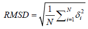
The quality of refined full length built model is assessed by RMSD between equivalent atoms in model and the native template structures after the optimal superposition of the two structures [14]. It can be summarized with an equation.
 (1)
(1)
Where δ is the distance between N pairs of equivalent atoms in the both structures i.e. refined Mtr model and template.
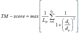
The TM-scoring function is a variation of Levitt–Gerstein (LG) score which depicts the structural similarity [11]. It can be depicted by the equation.
 (2)
(2)
Where LN is the length of the template structure, LT is the size of the aligned residues to the template structure, di is the distance between the ith pair of aligned residues and d0 is a scale to normalize the match difference. ‘Max’ denotes the maximum value after optimal spatial superposition. The value of the TM-score always lies between 0 and 1, with better templates having higher TM-scores.
The MaxSub score represents the similarity between two structures [15]. It identifies the maximum substructures which have Cα pairs <3.5Å of a model that superimpose ‘well’ over the experimental structure, and produces a single normalized score that represents the quality of the model.
The GDT-score is protein topology sensitive measure. It counts the number of Cα pairs which have a distance <1, 2, 4 and 8Å after the optimal superposition [12,13].
The Errat plot shows non-bonded interactions between different atoms types of the residues plotted as 9 residues sliding window. If the atoms of a structure are classified as carbon (C), nitrogen (N), or oxygen/sulfur (O), then this gives rise to six distinct interaction types (CC, CN, CO, NN, NO, and OO). The ith residue window is treated as a six-dimensional vector or observation ‘yi’.
 (3)
(3)
where, yi, represents the vectors of(interaction) spanning a nine-residue range centred on the ith residue.
The verify 3D determines the compatibility of built 3D model with its amino acid sequence by assigning a structural class based on its location and environment (alpha, beta, loop, polar, nonpolar, etc.) and comparing the results to good structures.
Comparison of refined Mtr homology model and template E. coli Gtr
Mtr and Gtr are homodimer enzymes with 459 amino acid residues. Mtr is also known as mycothiol disulfide reductase and belongs to oxidoreductase enzyme family that catalyse NADPH dependent reduction of mycothione to mycothiol. However, Gtr is FAD dependent enzyme that is categorized as oxidoreductase family of enzymes. Both the enzymes act as an antioxidant that save the bacterial cell from free radical damage and create reducing environment in the cell [49]. The Mtr refined homology model obtained through LM and template Gtr (1GER) were subjected to validation parameters. The validation statistics and their comparison with data already published for Mtr homology model by Lall et al. [29] is given in Table 1.
| Model validation statistics | |||
|---|---|---|---|
| Ramachandran plot | 1GER (template) | Refined Mtr | Mtr29 |
| % Amino acids in Favour region | 97.10 | 89.50 | 89.50 |
| % Amino acids in Allowed region | 2.90 | 7.00 | 8.30 |
| % Amino acids in outlier region | 0 | 3.50 | 1.80 |
| Errat overall quality factor | 97.50 | 96.00 | 96.00 |
| ProSA Z-score | -10.99 | -5.92 | -5.83 |
Table 1: Model validation comparative statistics of template and Mtr homology model.
We were able to successfully obtain model with quality similar to that of the published Mtr homology model. Although, the percentage residue in the disallowed region increases to 3.5% as compared to 1.8% in Mtr homology model (Table 1). Despite minor differences, the quality of the model obtained using LM method was comparatively reasonable. However, the model quality was not better than of the template 1GER in both the cases as seen in the Table 1 and Figure 1A.

Figure 1: ProSA Z-score comparison between (A) template 1GER and (B) refined Mtr homology model.
The Ramachandran plot statistics also showed wide differences between 1GER with 97.10% residues in the favour region and the Mtr model with only 89.5% in the same region. While no residues were observed in the outlier region of 1GER as compared to the two Mtr homology models. Similarly, the ProSA Z-score of the template model also showed a wide difference as observed in Table 1 and Figure 1B.
The 1GER template had a ProSA Z-score of ~-10.99 while the refined Mtr homology model scored ~-5.92. The black spot on the graph showed the template is of robust structural quality that falls exactly in region that is occupied by structures elucidated through X-ray crystallography technique. The refined Mtr model has a lower structural quality; however, it matches the structure elucidated by X-ray crystallography. Both the structures were within the range of scores typically found for native proteins of similar size. Similarly, the knowledge-based energy comparison also showed a wide difference in local model quality plot (Figure 2A).

Figure 2: Knowledge-based energy comparison between (A) template 1GER and (B) refined Mtr homology model.
As energy of single residue fluctuates a lot, therefore, the average energy of 40 residues (i+39) is assumed to be of 20th residue (i+19) and depicted as thick green line. Similarly, thin green line is signified an average energy of 10 residues (i+9). The positive values correspond to the erroneous part of the input structure while negative values correspond to the native fold of the protein structure. In the Figure 2B, template 1GER showed that the structure corresponds to the native fold of protein while the Mtr refined homology model showed only few parts corresponding to the native fold of protein.
The overall quality factor for Errat between template 1GER and refined Mtr model is easily comparable and similar as seen in the Table 1 and Figure 3A. On the error axis, the two lines in the plot show confidence limit with which structures are determining to be either acceptable or unacceptable. As observed in Figure 3B, few regions in the structure of template exceed the lower error limit while none of residues exceed the upper error limit. Similarly, the refined Mtr homology model showed few regions exceeding the lower error limit line while none of the residues exceeds the upper error limit bar.

Figure 3: Comparison of Errat plots between (A) template 1GER and (B) refined Mtr homology model.
Therefore, the quality of both the structures is comparable and the structures do not show sterically hindered region in the Mtr homology model.
Comparison of refined Mtr homology model
In our previous discussion, the refined Mtr homology model obtained using Errat-based LM method and template 1GER was compared. The LM involved twenty-five iterative steps to produce the final refined Mtr homology model. Therefore, during the process twenty-five structures were produced and analysed through validation parameters. Similarly, a MDS was performed for 75ns using an initial crude Mtr homology model and it produced twenty-five structures during the simulation at each step size of 3ns. In addition, refinement of model was performed using the 3Drefine, GalaxyRefine and FG-MD methods which utilized six steps to produce quality refined model. These structures were validated using the defined parameters to analyse the progress of refinement. Table 2 is showing the comparison of validation parameters for the final Mtr model obtained after refinement using various refinement techniques used in the present study.
| Model validation statistics | |||||
|---|---|---|---|---|---|
| Validation parameters | Refined final Mtr model from various techniques | ||||
| LM | MDS | GalaxyRefine | FG-MD | 3Drefine | |
| % residue in Favoured region | 89% | 90% | 94% | 80% | 91% |
| % residue in Allowed region | 7% | 8.1% | 5.3% | 14.9% | 5.7% |
| % residue in outlier region | 3.3% | 1.5% | 0.9% | 5.9% | 3.1% |
| Errat overall quality factor | 96% | 94% | 94% | 90% | 80% |
| ProSA Z-score | -5.9 | -7.4 | -8.08 | -8.10 | -7.8 |
| Verify 3D | 45% | 75% | 74% | 68% | 60% |
| RMSD* | 2.5Å | 2.5Å | 0.65Å | 0.65Å | 0.65Å |
| TM-Score | ~0.41 | ~0.42 | ~0.45 | ~0.45 | ~0.45 |
| MaxSub | ~0.084 | ~0.073 | ~0.084 | ~0.084 | ~0.084 |
| GDT-TS | 0.15-0.16 | 0.15-0.16 | 0.180-0.185 | 0.180-0.185 | 0.180-0.185 |
*alignment between template and refined Mtr model
Table 2: Comparative validation statistics for Mtr model obtained from various refinement techniques.
Comparison of Errat overall quality factor and Verify 3D: A comparison of Errat overall quality factors of generated structures during refinement process using various methods is given in the Figure 4A-E. It is observed in the LM plot that the overall quality factor gradually increases to about ~96% over the 25 steps (Figure 4A). However, as compared to LM, a steep increase in quality factor of about ~90 is observed during the first ~10ns of MDS (Figure 4B). It then remains between ~90% to ~94% for the rest of the simulations. Similar to MDS, GalaxyRefine and FG-MD methods are also showed steep increase in the overall quality factor ~90% and maintained at this point during refinement process.

Figure 4: Comparison of Errat-overall quality factor during refinement process using various methods.
Also, 3Drefine method showed steep increase to ~85%, however, it gradually decreases to ~80%. Analysis of the Errat overall quality factor clearly indicates that MDS, GalaxyRefine and FG-MD are superior methods that produce quality model as compared to LM and 3Drefine methods. Also, all three methods are based on the molecular dynamics strategy that indicates the effectiveness of these methods in refining the model (Figure 5A-E).
In contrast to Errat plot, verify 3D shows different pattern during refinement process in LM and 3Drefine. It gradually decreases from ~65% to ~45% and 60% for LM and 3Drefine respectively (Figure 5A-C). This indicates that Errat-based refinement does not correspond to improvement of 1D-3D compatibility throughout refinement using LM and 3Drefine. Nevertheless, both methods produce a reasonable refined Mtr homology model by end of refinement process with a >50% 1D-3D compatibility. On the other hand, the MDS shows a smooth pattern of curve in verify 3D plot (Figure 5B). It produces Mtr homology model with ~75% 1D-3D compatibility by the end of 75ns simulation. Similar to Errat plot, GalaxyRefine and FG-MD show steep increase in percentage 1D-3D compatibility during refinement process (Figure 5D and 5E). However, similar to MDS, GalaxyRefine reaches to ~74% while FG-MD remains at ~68% 1D-3D compatibility. The verify 3D shows a pattern corresponding to Errat plot for MDS, GalaxyRefine and FG-MD that producing the refined Mtr homology model, with ≥ 70% 1D-3D compatibility.

Figure 5: Comparison of verify 3D using various refinement methods.
Dihedral angle-based distribution of residues in Ramachandran plot Residue distribution in favoured region: The favoured region of Ramachandran plot accommodates residues belonging to the secondary structure of a protein that accounts for maximum number of residues in that region. In the Figure 6A, the percentage of residue in favoured region decreases from ~92% to ~89 by the end of refinement process using LM method. Corresponding to this, the number of residues also decreases from 420 to 410 (Figure 6a). It shows the mobilization of residues to one or another region of Ramachandran plot due to flexible dihedral angles. As observed in LM method, the percentage of residue decreases in the favoured region during Mtr homology model refinement using MDS method (Figure 6B). The number of residues also decreases from 420 to 413 (Figure 6b).

Figure 6: Distribution of residues in favoured region.
However, as compared to LM method, few residues are mobilized to other region of Ramachandran plot. Similar to MDS, percentage of residue decreases in 3Drefine from ~92% to 91% and remains stable at ~91% throughout the refinement process with decrease of 420 to 417 residues (Figure 6C, 6c). However, a steep decrease in percentage of residues from ~92% to ~80% is observed for FG-MD corresponding to decrease in residues from 420 to 362 residues (Figures 6D, 6d).
Only, GalaxyRefine shows increase in percentage residues from ~92% to ~94% and remains stable at ~94% (Figures 6E, 6e). Similarly, residues increase from 420 to 420 in the favoured region of Ramachandran plot.
Thus, MDS, 3Drefine and GalaxyRefine methods are better in retaining more residues in favoured region, though, the number of residue curve does not show smooth pattern in MDS as seen in case of LM, 3Drefine and GalaxyRefine methods. The MDS and GalaxyRefine method show that they are more effective than other methods for structural refinement of homology model as they could accommodate more number of residues in the favour region.
Residue distribution in allowed region: Generally, the allowed region of the ramachandran plot accommodates residues that belong to left-handed α-helices and beta sheets. It is observed that the percentage of residue increases in the allowed region from 5.3% to 7% during refinement process using LM method (Figure 7A). Correspondingly, the numbers of residues also increase in the allowed region from 24 to 32 (Figure 7a). This is in agreement with our previous discussion where it was observed that the percentage and number of residues decrease due to mobilization of residues into another region of Ramachandran plot. During the refinement process using MDS, percentage and number of residues increase from 5.3% to 8.1% and 24 to 37 respectively (Figures 7B, 7b), which are similar to that of LM.

Figure 7: Distribution of residues in allowed region.
However, as compared to MDS described in the previous section, mobilization of residues from favoured to the allowed region is more in the case of LM. It clearly indicates that residues would have mobilized from outlier region to allowed region in case of MDS. Similarly, in FG-MD method, percentage and number of residues increase from 5.3% to 14.9% and 24 to 68 respectively (Figures 7E, 7e).
It indicates that residues would have mobilized from favoured and outlier region to allowed region in case of FG-MD. In case of 3Drefine, the percentage and number of residues increase from 5.3% to 5.7% and 24 to 26 respectively (Figures 7C, 7c). While in case of GalaxyRefine, percentage and number of residues do not show variation (Figures 7D, 7d). It is because that most of the residues remain accommodated in favoured region during refinement using GalaxyRefine. This indicates that MDS and GalaxyRefine are superior method for structural refinement as they effectively make the residues either to mobilize into allowed region or accommodated in the favoured region leaving a very few in outlier region.
Residue distribution in outlier region: The outlier region of the Ramachandran plot is termed as forbidden or disallowed region. Generally, in addition to other residues, this region could have glycine and proline residue [50]. The glycine has no β-carbon i.e. no side chain, and therefore, it is least sterically hindered among all amino acid residues and consists of enormous dihedral angle flexibility. So, glycine frequently occurs in turn regions of proteins where any other residue would be sterically hindered. On the other hand, proline contains cyclic side chain and, therefore, rotation around the bond is most constrained among all other residues. In addition to this, many residues belong to the loop regions that may be mobilized into outlier region. In the outlier region, the percentage residue increases from 2.8% to 3.3% in case of LM (Figure 8A). Similarly, the number of residues also increases from 13 to 15 (Figure 8a).

Figure 8: Distribution of residues in outlier region.
Thus, in addition to the allowed region, residues mobilize from the favoured to outlier region in refinement process using LM method. However, the percentage of residue decreased from 2.8% to 1.5% in case of structural refinement using MDS method (Figure 8B). Similarly, numbers of residues also decrease from 13 to 7 (Figure 8b). In 3Drefine method, percentage and number of residues increase in outlier region from 2.8% to 3.1% and 13 to 14 respectively (Figures 8C, 8c).
Similarly, in FG-MD method, percentage and number of residues increase in outlier region from 2.8% to 5.9% and 13 to 27 respectively (Figures 8E, 8e). Opposite to this, in GalaxyRefine, percentage and number of residue decrease in outlier region from 2.8% to 0.9% and 13 to 4 respectively (Figures 8D, 8d).
In MDS and GalaxyRefine methods, residues are mobilized to the favoured as well as allowed region leading to less number of residues in outlier region. It produces a Mtr model with least structural error. Thus, it proves that MDS and GalaxyRefine are more effective methods to refine and produce a homology model with reasonable stereo-chemical structural quality.
Comparison of ProSA Z-score-based overall model quality
ProSA is an important method to evaluate homology model quality based on the calculated z-score. It indicates overall model quality that is displayed in a plot containing the z-scores of all experimentally determined protein in PDB. It can be used to check whether the z-score of the input structure is within the range of scores typically found for native proteins of similar size. A higher z-score for a homology model is interpreted as a better-quality model. In Figure 9A, the overall model quality of Mtr model decreases gradually during the refinement process using LM method, as the z-score decreases from ~-7.8 to ~-5.9. Similarly, the overall model quality also decreases as z-score diminishes a little from ~-7.8 to ~ -7.4 in case of MDS (Figure 9B). However, 3Drefine method shows retention of z-score to ~7.8 throughout the refinement process (Figure 9C). Opposite to this, GalaxyRefine and FG-MD methods show a little increase in z-score from ~-7.8 to ~-8.08 and ~-8.10 (Figures 9D and 9E).

Figure 9: The z-score based overall model quality comparison throughout the refinement process using various methods.
It shows that GalaxyRefine and MDS are effective methods for the refinement of Mtr homology model as compared. In addition, 3Drefine and FG-MD also perform reasonably to produce quality z-score Mtr model.
Similarity based evaluation of the refined Mtr model using RMSD, TM-score, MaxSub score and GDT-TS score
The similarity between template and built homology model is important parameter to evaluate the exact structural fold. In absence of native structure of Mtr, we have carried out the comparison with template, assuming it as a native structure. The first data point in the graph generally representing the native data point set which is compared with data set of predicted refined Mtr structures (Figure 10A-E).

Figure 10: Calculation of RMSD between template and built refined Mtr homology model.
The RMSD is one of the best and simple approaches to evaluate the backbone and side chain differences. However, TM-score, MaxSub score and GDT-TS score are more rigorous parameters to evaluate the same protein fold available in template and homology model. In case of LM and MDS, RMSD is observed about 2.5Å in the end of refinement process (Figures 10A and 10B). It shows very little differences in the superposition of the Cα-backbone chain of template and refined model.
However, 3Drefine, GalaxyRefine and FG-MD show even very little differences of about ~0.65Å in superposition of Cα-backbone between template and refine model in the end of refinement process. It clearly indicates that later three methods are more effective in keeping the protein fold of refine model in the position as of template.
Similarly, TM-score shows the same pattern as of RMSD. It is observed about ~0.45 in case of 3Drefine, GlaxyRefine and FG-MD (Figure 11A-E). It signifies that protein fold of refined model is in the same fold as of template. However, TM-score for LM and MDS is found about ~0.41 and ~0.42 that indicates towards a difference in backbone superimposition (Figures 11A and 11B).

Figure 11: Comparison of TM-score used for similarity of protein folds.
MaxSub score also indicates the fold similarity between the template and the homology model. And, it is calculated unity for the exact protein fold similarity. In case of MDS, it is found to be ~0.073 that signifies low fold similarity (Figures 12A and B).
In case of LM, 3Drefine, GalaxyRefine and FG-MD, MaxSub score is observed about ~0.084 (Figure 12A-E). However, in all the cases, this score indicates very low similarity among the folds but later one still performs well.

Figure 12: Comparison of MaxSub score used for protein fold similarity.
GDT-TS score shows the pattern similar to MaxSub score. In case of MDS, GDT-TS score is observed between 0.15 to 0.16 that signifies low fold similarity between template and refined Mtr model (Figure 13A). Similarly, LM also shows the low fold similarity (Figure 13B). However, in case of 3Drefine, GalaxyRefine and FG-MD; GDT-TS score is found between 0.180 to 0.185, which show comparatively better fold similarity of Mtr model as compared to LM and MDS (Figure 13C-E).

Figure 13: GDT-TS score for fold similarity between template and refined Mtr homology model.
The protein fold similarity is observed little low in all cases however, it is found reasonably better in case of GalaxyRefine and FG-MD. It can be inferred from the discussion that both methods are inspired by molecular dynamics which takes the opportunity to refine the Mtr model little better than any other methods used in the study.
Secondary structure comparison
The secondary structure of protein consists of α-helix, β-sheet, 3-10 helix and Π-helix. These secondary structures are responsible for forming the core structure of protein 3D architecture. In the Figure 14A-E, a comparison of secondary structure of Mtr homology model is depicted throughout the refinement process. It is observed that some secondary structures present in MDS, 3Drefine, GalaxyRefine and FG-MD are missing in LM. The missing secondary structures are highlighted by red colored rectangular boxes marked with a, b, c, d, e, f, and g. The box “a” shows a very short stretch of β-sheet (residue 105- 108) that gets converted to turn while it remains as β-sheet in MDS, 3Drefine, GalaxyRefine and FG-MD.

Figure 14: Comparison of secondary structure after refinement of Mtr homology model using (A) LM, (B) MDS, (C) 3Drefine, (D) GalaxyRefine and (E) FG-MD methods.. The missing secondary structures are marked with red colored rectangular boxes and notified as a, b, c, d, e, f, and g for the comparison throughout refinement process.
The box “b” shows a stretch of α-helix (residue 181-194) which converted to coil. Similarly, box “c” shows another stretch of α-helix (residue 212-225) which also converts to coil. However, both stretch “b” and “c” remain as α-helices in MDS, 3Drefine, GalaxyRefine and FG-MD.
A short stretch of α-helix (residue 275-278) shown in box “d” is converted to coil. However, this stretch remains as α-helix in 3Drefine while it gets converted into 3-10 helices in MDS, GalaxyRefine and FG-MD.
A short stretch of turn (residues 346-349 and 376-379) depicted by boxes “e” and “f” are converted into coil. However, these stretches remain as turn in the in MDS, 3Drefine, GalaxyRefine and FG-MD.
And only a small turn depicted as box “g” is converted into secondary structure β-sheet. However, it remains as turn in the MDS, 3Drefine, GalaxyRefine and FG-MD. When the secondary structure represented in Figure 14A-E is compared, structure marked in boxes in Figure 14B-E are found to maintain their native topology.
It shows that MDS, 3Drefine, GalaxyRefine and FG-MD methods are more effective to restore the native protein topology as compared to LM method where some secondary structures and a turn convert to other structural motifs.
The observed topology differences in Mtr homology model is also seen after refinement using LM, MDS, 3Drefine, GalaxyRefine and FG-MD methods (Figure 15A-E). Therefore, topological differences observed in secondary structure plot in Fig 14 are completely in agreement with 3D structural differences observed in Figure 15. It shows that secondary structures of Mtr homology model are more propelled to be converted during structure refinement using LM method while the native topology of Mtr homolog model is conserved during refinement process using MDS, 3Drefine, GalaxyRefine and FG-MD methods.

Figure 15: Comparison of secondary structure topology after refinement using (A) LM, (B) MDS, (C) 3Drefine, (D) GalaxyRefine and (E) FG-MD methods. The structures marked with, the blue circles highlight structures that disappear during refinement process.
Mtr homology model was built using MODELLERv9.16 program with Gtr (1GER, E. coli glutathione reductase) as the template. A single Mtr model was picked up among the ten built models based on low molpdf and DOPE scores. The model was refined using different methods: LM, MDS, 3Drefine, GalaxyRefine and FG-MD. Initially, a comparison of Gtr template and the refined model was presented to describe the structural quality of the template.
The Mtr homology model was refined using LM, MDS, 3Drefine, GalaxyRefine and FG-MD methods. Errat overall quality factor for LM and MDS methods was increased. The overall quality factor increased gradually to ~96 in case of LM while a steep increment is seen from ~65 to ~95 in case of MDS during the first 10ns of simulations. Similarly, GalaxyRefine and FG-MD methods also showed steep increase in the overall quality factor to ~90% while 3Drefine method showed steep increase to ~85%. The verify 3D showed the 1D-3D compatibility decreasing from ~65% to ~53% in LM while compatibility was observed to increase from 65% to ~75% in MDS method. Similar to MDS, GalaxyRefine reached to ~74% while FG-MD remained at ~68% 1D-3D compatibility.
The analysis of dihedral angle distribution based Ramachandran plot showed residues in favour decrease and mobilized into the allowed and outlier region during refinement using LM method. Therefore, increase in the allowed and outlier region where less numbers of residues are expected. However, residues from favour and outlier regions were found to decrease and mobilized into allowed region during refinement process using MDS method. This led to decrease in the number of residues in the outlier region. Similar to MDS, GalaxyRefine showed mobilization of residues from Allowed and outlier regions to favoured region. However, in case of 3Drefine and FG-MD, residues were observed to mobilize into outlier regions.
The ProSA z-score based overall model quality was compared throughout the refinement process using LM and MDS methods. The z-score decreases gradually from ~-7.8 to ~-5.8 in LM method, whereas the z-score in MDS method score decreased very little from ~-7.8 to ~-7.4. Opposite to this, 3Drefine, GalaxyRefine and FG-MD showed increase in z-score about ≥ -8. Similarity based evaluation showed RMSD ≤ 0.6Å in case of 3Drefine, GalaxyRefine and FG-MD whereas, LM and MDS showed RMSD ≥ 2.5Å. TM-Score also observed to about ≥ 0.45 in case of 3Drefine, GalaxyRefine and FG-MD as compared to ~0.43 in case of LM and MDS. GDT-TS and MaxSub scores showed similar pattern. In case of MDS, GDT-TS and MaxSub scores signifies low fold similarity between template and refined Mtr. Similarly, LM also shows the low fold similarity. However, in case of 3Drefine, GalaxyRefine and FG-MD, these scores showed comparatively better fold similarity of Mtr model as compared to LM and MDS
Topology comparison was carried out and few secondary structures in Mtr homology model were found to convert into coil or another motif during the refinement process using LM method. However, in case of MDS, 3Drefine, GalaxyRefine and FG-MD methods, the topology of Mtr homology model was stable and retained its native conformation during the refinement. This study solely depicts a comparison of the structure refinement methods emphasizing on MD-based techniques to be used for structural refinement.