International Journal of Advancements in Technology
Open Access

Brain Stroke Classification Using Ensemble Learning Approaches

Houmem Slimi^* and Sabeur Abid ^*Correspondence: Houmem Slimi, Department of Artificial Intelligence, Laboratory of Signal, Image processing and Energy Mastery (SIME), Higher National School of Engineers (ENSIT), University of Tunis, Tunisia, Email:

Author info »

Introduction

Brain stroke is a serious medical issue that needs to be identified and treated right away to have the least number of negative effects on the patients' health. For efficient treatment planning and patient management, it is essential to classify stroke types accurately and promptly. Machine learning techniques have become effective research tools in the field of medicine, with the potential to improve stroke classification efficiency and accuracy. Large amounts of medical data, including clinical records, patient demographics and brain imaging scans, can be analyzed by machine learning algorithms to find trends and make predictions. These algorithms can be taught to distinguish particular traits and qualities connected to various stroke types by being trained on labeled datasets. As a result, they may categorize new instances in accordance with the discovered patterns, assisting healthcare providers in making defensible choices. For the classification of strokes, supervised learning, unsupervised learning, and deep learning have all been investigated. Support Vector Machines (SVM) and random forests are examples of supervised learning algorithms that can be trained on labeled data to categorize strokes into preset groups, such as ischemic stroke, hemorrhagic stroke or Transient Ischemic Attack (TIA). In stroke data, latent patterns can be found using unsupervised learning algorithms, such as clustering methods, which may uncover novel subtypes or variations. Convolutional Neural Networks (CNN), for example, are deep learning models that can accurately classify different types of strokes by extracting complex characteristics from medical images. There are many advantages to employing machine learning for stroke classification. It can help medical personnel identify patients more quickly and accurately, leading to prompt interventions and better patient outcomes. The ability of machine learning algorithms to effectively handle massive datasets also makes it possible to analyze a variety of patient groups and find brand-new stroke subtypes. The development of individualized treatment plans and a greater understanding of stroke pathogenesis may result from this.

In a study by Gupta et al. [1], the comparison of all machine learning methods is realized. Following a thorough analysis of the data, it was discovered that the AdaBoost, XGBoost and Random Forest Classifiers had the lowest percentages of inaccurate predictions and the highest accuracy ratings, with 95%, 96% and 97%, respectively.

The hybrid system suggested in a study of Bathla et al. [2], found a condensed collection of characteristics that might accurately predict brain stroke. A feature reduction ratio of 36.3% was supplied by FI. The hybrid system with the highest accuracy of 97.17% for predicting brain strokes uses FI as the feature selection method and RF as the classifier.

In comparison to a single classifier, the suggested soft voting approach proposed by Srinivas et al. [3] increased final prediction accuracy and resilience. In order to increase classification accuracy, a swarm intelligence-based optimization was developed. The proposed model had a 96.88% accuracy rate.

Lu, et al. [4] used a portable eye-tracking equipment and recorded the eye movement signals and computed eye movement features by combining traditional Chinese medicine theory with contemporary color psychology ideas. Gradient Boosting Classifier (GBC), XGBoost and CatBoost were used to further train the stroke identification models based on eye movement characteristics. Random Forest (Rf), K-Nearest Neighbors (KNN), Decision Tree (DT) and Random Forest (RF) were also used. The models that were trained using eye movement traits performed well in identifying stroke victims, with accuracies ranging from 77.40% to 88.45%. With a recall of 84.65%, a precision of 86.48% and an F1 score of 85.47% under the red stimulus, the eye movement model trained by RF emerged as the top machine learning model.

Materials and Methods

Our study was based on brain stroke’s data from Kaggle. We concentrated on participants who were over the age of 18 from this dataset. The total participant count was 4981 and all of the qualities (10 used as input into ML models and 1 for the target class) are specified as follows:

Inputs: Gender, age, hypertension, heart disease, ever married, work type, residence type, avg glucose level, BMI, smoking status.

Output: Stroke.

With the exception of the age, average glucose level and BMI, other characteristics are nominal. Table 1 gives an idea about our dataset.

Table 1: Brain stroke dataset.

Data comprehension

In classification analysis, feature significance is a crucial element that makes it easier to create high-fidelity, correct ML models. The classifiers get more accurate as more features are taken into account. If irrelevant features are taken into account when training ML models, their performance may suffer. The technique of giving each feature in a dataset a score is known as feature ranking.

In this manner, the most important or pertinent ones are taken into account, namely those that may significantly contribute to the target variable to improve the model's accuracy. Table 2 shows the significance of the dataset features in relation to the stroke class. A random forest classifier is used to determine a ranking score.

Table 2: Features importance of the balanced data.

Data preprocessing

One hot encoding is a technique used to transform features values (in our case: Gender, age, ever married, work type, residence type, smoking status) into numeric values. We realize this step in order to divide dataset into train and test parts [5].

The dataset contains 2 classes: Stroke and no stroke. According to data, 248 patients belong to class1 (stroke) and 4733 belong to class 2 (no stroke), so there is clearly a problem of imbalanced classes. Figure 1 shows a comparison between the two classes.

We choose oversampling technique called SMOTE [6] to solve this problem. Figure 2 shows results of this strategy. We choose to split data as 80% for train and 20% for test.

Figure 1: Imbalanced classes histogram.

Figure 2: Balanced classes histogram after using SMOTE.

Machine learning algorithms

Multilayer Perceptron (MLP): A fully linked feed forward Artificial Neural Network (ANN) is referred to as a Multilayer Perceptron (MLP). The back propagation learning process is used to train the MLP's neurons. MLPs can tackle problems that are not linearly separable and are made to approximate any continuous function [7,8].

XGBoost: The supervised learning field includes the boosting technique XGBoost, which is an ensemble approach based on gradient boosted trees [9]. Through a serial training procedure, it combines the predictions of "weak" classifiers (tree models) to produce a "strong" classifier (tree models). By including a regularization term, it can prevent over-fitting. The learning process is accelerated by parallel and distributed computing, resulting in a quicker modeling process [10].

AdaBoost: The Adaboost algorithm can be stated as follows: In the first step, several weak classifiers are trained using the same training data; in the second step, the weak classifier set transforms into a stronger strong classifier. The weight algorithm of the samples is set according to whether the training classification is accurate and the distribution of the correct rate prior to training and the effect is produced by altering the data distribution. Based on this, the revised new weights are distributed to the lower-level classifiers for ongoing training and finally, the numerously trained classifiers are integrated to create the final decision classifier [11].

K Nearest Neighbor (KNN): KNN or k nearest neighbor classifications, uses a combination of K's most recent historical data to identify new records. Over the past 40 years, KNN has undergone extensive research in the field of pattern recognition. The KNN principle is as follows: First, determine the distance between the new sample and the training sample and then locate the K closest neighbors. Next, choose the category to which each neighbor belongs and if all of them do, the new sample will also fall into that category. If not, each post-selection category is scored and the new sample category is chosen in accordance with predetermined guidelines [12].

Stacking: Stacking [13] is an ensemble learning technique that makes use of a number of heterogeneous classifiers, the predictions of which are then concatenated to create a metaclassifier. The meta-model was trained using the outputs of the base models, whereas the base models were trained using the training set. In this study, the basis classifiers employed in the stacking ensemble include multilayer perceptron, XGBoost, AdaBoost and the random forest meta-classifier was trained using the predictions from these classifiers.

Evaluation metrics: Several performance indicators were logged during the consideration and evaluation of the ML models. The most frequently utilized in the pertinent literature will be taken into consideration in the current study [14].

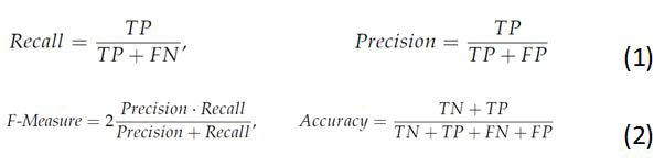
The proportion of people who had a stroke and were correctly identified as positive, relative to all positive participants, is known as recall (also known as true positive rate) or alternatively, sensitivity. When working with imbalanced data, precision and recall are more suited to identifying a model's faults. The precise number of stroke victims who genuinely fall into this category is shown. Recall reveals how many stroke victims were anticipated properly. The predictive performance of a model is summed up by the F-measure, which is the harmonic mean of the precision and recall.

As you can see, TP stands for true positive, TN for true negative, FP for false positive and FN for false negative.

An effective metric with values between (0, 1) is the Area Under the Curve (AUC).

The ML model performs better in separating stroke from nonstroke events the closer it gets to one. The AUC is equal to one since there is perfect discrimination between instances of the two classes. On the other hand, the AUC is equal to 0 when all non-strokes are categorized as strokes and vice versa.

Results and Discussion

In this part, we use Kaggle platform with GPU P100 service for training and testing our proposed model to increase the running time of our code. The computer used for the experiments includes the following features: Windows 10 Professional, 64-bit operating system, Intel(R) Core(TM) i7-8750H CPU @ 2.20 GHz 2.21 GHz 8 GB Memory, x64-based processor. GridSearchCV was used in our stacking model on the balanced dataset of 9466 occurrences. Four basis classifiers were integrated for the stacking model's implementation.

To be more precise, the results of Multilayer Perceptron, XGBoost, AdaBoost and KNN were chosen and fed into a Random Forest meta-classifier. The MLP model was configured as follows: Activation='tanh' and learning rate was set to 0.001. In terms of the XGBoost, the learning rate was fixed to 0.1 and n_estimators was 200. Same parameters were set to Adaboost. Finally, KNN was utilized with n_neighbors equal to 3 and ‘distance’ as function for weights.

In all criteria taken into consideration, the stacking with GS model underneath the chosen base models was the most effective. According to Table 3, the uses of GridSearchCV increase all parameters of stacking model by approximately 2%. Similar to the XGBoost classifier, the voting classifier also produced high results. Focusing on the AUC measure, the stacking with GS and XGBoost models have almost comparable discriminating capabilities, which demonstrate that both models can successfully distinguish the instances of stroke from nonstroke with a high probability of 98.6% and 98.1%, respectively.

Table 3: Average performance of ML models.

The voting model comes third, after stacking and XGBoost and has a relatively high AUC of 97.2%. Figure 3 shows a comparison between previous models in term of confusion Matrix.

Figure 3: Confusion matrix of used models.

According to Figure 3, the best model is XGBoost (because it contains less FP and FN rates), the second is Voting model and the third is our Stacking model. Figure 4 illustrates the importance of Using GS to improve evaluation metrics of Stacking model.

Figure 4: Confusion matrix of Stacking model without GS and with GS.

Conclusion

A stroke is a life-threatening condition that needs to be avoided and/or treated in order to prevent unanticipated complications. The clinical providers, medical specialists and decision-makers can now take advantage of the existing models to find the most pertinent aspects (or alternatively, risk factors) for the occurrence of strokes and can evaluate the corresponding probability or risk.

In this regard, machine learning can help with the early diagnosis of stroke and lessen its severe aftereffects. This study combines the use of EL techniques like Boosting (XGBoost, AdaBoost), Bagging (Random Forest) and Stacking (using Random Forest as a meta-classifier) and examines the efficacy of multiple ML algorithms to determine the best reliable algorithm for stroke prediction based on a number of variables that capture the profiles of the participants.

The models' interpretation and the classifiers' classification performance are mainly supported by the performance evaluation of the classifiers using AUC, F-measure (which summarizes precision and recall) and accuracy. Additionally, they demonstrate the models' reliability and prognostication power for the stroke class. With an AUC of 98.6%, F-measure, precision, recall and accuracy of 98.4%, stacking classification with GS performs better than the other approaches.

References

1. Gupta S, Raheja S. Stroke prediction using machine learning methods. In 2022 12th International Conference on Cloud Computing, Data Science and Engineering (Confluence) 2022; (pp. 553-558). IEEE.

   [Crossref] [Google Scholar]

2. Bathla P, Kumar R. A hybrid system to predict brain stroke using a combined feature selection and classifier. Intel Med. 2024;4(02):75-82.

   [Google Scholar]

3. Srinivas A, Mosiganti JP. A brain stroke detection model using soft voting based ensemble machine learning classifier. Measure Sensor. 2023;29:100871.

   [Crossref] [Google Scholar]

4. Qingya Lu, Jingyuan Deng, Ying Yu, Yang Li, Kunni Wei, Xia Han, et al. Machine learning models for stroke detection by observing the eye-movement features under five-color visual stimuli in traditional Chinese medicine. J Trad Chinese Med Sci. 2023;10(3):321-330.

   [Crossref] [Google Scholar]

5. Rodríguez P, Bautista MA, Gonzalez J, Escalera S. Beyond one-hot encoding: Lower dimensional target embedding. Image Vision Comput. 2018;75:21-31.

   [Crossref] [Google Scholar]

6. Maldonado S, López J, Vairetti C. An alternative SMOTE oversampling strategy for high-dimensional datasets. Appl Soft Comput. 2019;76:380–389.

   [Crossref] [Google Scholar]

7. Abirami S, Chitra P. Energy-efficient edge based real-time healthcare support system. Adv Comput. 2020;117(1):339–368.

   [Crossref] [Google Scholar]

8. Shankar K, Zhang Y, Liu Y, Wu L, Chen CH. Hyperparameter tuning deep learning for diabetic retinopathy fundus image classification. IEEE Access. 2020;8:118164–118173.

   [Crossref] [Google Scholar]

9. Chen T, Guestrin C. Xgboost: A scalable tree boosting system. InProceedings of the 22nd acm sigkdd international conference on knowledge discovery and data mining 2016, pp. 785-794.

   [Crossref] [Google Scholar]

10. Kameda H, Nomoto K, Kosuge Y, Kondo M. Target tracking algorithm in radar reference coordinates using full-coupled filters. Electronics and Communications in Japan, Part 1: Communications. 1997;80(7):90-98.

    [Crossref] [Google Scholar]

11. Jia‐qiang L, Rong‐hua Z, Jin‐li C, Chun‐yan Z, Yan‐ping Z. Target tracking algorithm based on adaptive strong tracking particle filter. IET Sci Measure Technol. 2016;10(7):704-710.

    [Crossref] [Google Scholar]

12. Wang L. Research and implementation of machine learning classifier based on KNN. Mater Sci Eng. 2019;677(5):052038.

    [Google Scholar]

13. Rajagopal S, Kundapur PP, Hareesha KS. A stacking ensemble for network intrusion detection using heterogeneous datasets. Secur Commun Netw. 2020;2020(1):4586875.

    [Crossref] [Google Scholar]

14. Hossin M, Sulaiman MN. A review on evaluation metrics for data classification evaluations. Int J Data Min Knowl Manag Proc. 2015;5(2):1.

    [Google Scholar]