Journal of Geology & Geophysics
Open Access
ISSN: 2381-8719
ISSN: 2381-8719
Research Article - (2014) Volume 3, Issue 6
Droughts are common natural phenomenon in Ethiopia which has been affecting food insecurity and imposing other complex problems. Severe droughts happened once every 10 years in the north and north east Ethiopia, now becoming more frequent and covering areas that never experience drought before, in the southern parts of the country. According to IPCC droughts will become more intense, frequent and severe in the future due to the impact of climate change. This thesis presents the assessment of projected impact of climate change on hydrological drought in the Lake Tana basin in Ethiopia, which is the headwater for the Blue Nile River. The rainfall-runoff HBV model was calibrated and validated against historical data to obtain a reference situation to the possible impact of climate change on hydrological drought in four sub-basins and the Lake Tana basin. Datasets obtained from the EU- ATCH project for three General Circulation Models (CNCM3, IPSL and ECHAM) were used as an input to the HBV model, which was recalibrated for the same historic period to obtain an assessment to what local downscaled, bias-corrected GCM can be used as a forcing data for hydrological drought assessment. Next the GCM outputs with the recalibrated HBV model were used to simulate future streamflow for two future time windows (2021-2050 and 2071-2100) and for one future emission scenario A2. The variable threshold level method combined with a 10-day moving average streamflow was used to detect hydrological drought characteristics.
Keywords: Climate change; Hydrological drought; GCMs; Threshold levle method; HBV; Lake Tana basin
In the rainy season (JJAS) at which the basin gets more than 70 to 90% of the total rain, the precipitation is projected to increase by about 2.6% and 5.7% for ECHAM and IPSL, respectively, while CNCM3 predicts a reduction in precipitation by about 5.8% for the intermediate future. All models projected that the mean temperature will increase in most months of the year for both intermediate and far future periods. At the end of the 21st century both ECHAM and IPSL project an increase in precipitation by about 3.5% and 5.8% respectively. Comparison of drought characteristics derived from observed data with that derived from GCMs for the reference situation revealed that, the number of drought derived from all GCMs is smaller than the number of droughts simulated using observed data for the historical period, in the Lake Tana basin. Both ECHAM and CNCM3 underestimated the number of droughts by 38%, and IPSL by about 68%. CNCM3 and ECHAM overestimated the average drought duration by 47% and 49% respectively. The average deficit volume is overestimated for all GCMs. In most of sub-basins the percentage difference in the number of droughts revealed that the number of droughts using ECHAM forcing has relatively small values. This suggests that ECHAM could be the best model that could be used to analyze number of droughts in the basin. The climate change impact assessment revealed that, according to CNCM3, the number of droughts in the Lake Tana basin is expected to increase by 100% and 68.8% in the intermediate and far future, respectively. IPSL projected a decrease in the number of streamflow drought by 35% for the intermediate and far future. ECHAM projected also projected a decrease in the number of streamflow drought by 16% and 28% for intermediate and far future, respectively. The average drought duration is projected to reduce in the intermediate and far future periods for both CNCM3 and ECHAM. For example, in case of the Lake Tana basin, IPSL projected an increase in the average drought duration by 80 and 95% for the intermediate and far future respectively. CNCM3 projected a decrease in average drought duration by 36 and 48% for the intermediate and far future, respectively. According to ECHAM the average drought duration in the Lake Tana basin projected to reduce by 42 and 21%, respectively. At the end of the 21st century, the deficit volume also projected to decrease by about 33 and 2% for CNCM3 and ECHAM respectively. For the IPSL model, the deficit volume is expected to increase by 9 and 19% respectively, for the intermediate and far future periods. There is no consensus in the direction and magnitude of change in hydrological drought characteristics from one basin to another for the same GCM this could be due to the relative large variability across sub-basins with respect to climate, topography and physiographical or hydrological characteristics. There is also large difference in the direction and magnitude of change of drought characteristics among GCMs in the same basin or sub-basin. The variation among the GCMs is due to the fact that different climate models exhibit a wide range of climate sensitivities. Climate change is likely to happen with surface temperatures having increased by about 0.74°C from 1906 to 2005 [1]. Observations show that there are changes in precipitation, occurring in the amount, intensity, frequency and type of precipitation, as a result of direct influences of climate change. In both the developed and developing world, climate impacts are reverberating through the economy, threatening water availability, hydro-power generation, extreme weather impacts, sea level rise, amongst others [2]. The underdeveloped and poor countries that are most vulnerable bearing the greatest impacts of climate change [1]; East Africa/N-East Africa is amongst the most vulnerable regions to climate change impacts since economic growth in these countries is strongly weather dependent, ranging from rain-fed agriculture, to pastoral activities. According to a UNDP report, agriculture accounts for around 60% of overall employment in some countries and more than 50% of GDP [3]. There have been notable droughts in Ethiopia throughout human [4]. Previous droughts and the frequency of rainfall deviation from the average suggest that droughts occur every 3-5 and 6-8 years in northern Ethiopia and every 8-10 years for the whole country [4]. The Lake Tana basin has been identified as an economic ‘growth corridor’ by the Government of Ethiopia and the World Bank. The intention is to stimulate economic growth and reduce poverty through the development of hydropower and a number of irrigation schemes [5,6].
According to the Fourth Assessment Report released by the Intergovernmental Panel on Climate Change, droughts have become longer and more intense, and have affected larger areas since the 1970s; the land area affected by drought is expected to increase and water resources availability in affected areas could decline as much as 30% by mid-century. Drought is defined as a sustained and regionally extensive occurrence of below average natural water availability and may affect all components of the water cycle [7]. This can be characterized by a deviation from normal conditions of the physical systems, which is reflected in variables such as precipitation, soil water, ground water and streamflow. The primary cause of drought is a lack of precipitation over a large area and for an extensive period of time that propagates through the hydrological cycle and gives rise to different types of drought [7]. As a result of its significant water resources potential, the Lake Tana basin is at the core of Ethiopia’s plans for economic development. A number of schemes are planned for the near future. Three hydropower plants are operational in the Lake Tana basin: Tana–Beles, Tis Abbay I and II. In addition, a number of irrigation schemes (approximately 70,000 ha) are planned on the main rivers flowing into the lake and around the lake itself [8]. Assessment of impact of climate change on hydrological drought in the basin is very essential for effective water management for the hydropower generating plants and irrigation activities. This study investigates the impact of climate change on hydrological drought in the Lake Tana basin. Climate change projections were used from three General Circulation Models and for A2 scenario. Climate change and variability has potential impact in Africa in general and East Africa in particular on different natural resources, such as water availability, which in turn greatly influences agriculture, energy, ecosystems and many other sectors. Even in the absence of climate change, the present population trends and patterns of water use indicate that more Africa countries will exceed the limits of their economically usable, land-based water resources before 2025 [1]. A projected increase in rainfall in East Africa, extending into the Horn of Africa, is robust across an ensemble of models of which 18 out of 21 models project an increase in the core of this region, east of the Great Lakes [1]. Local and regional changes in the character of precipitation further depend on atmospheric circulations, which are in turn associated to climate change. For example, rainfall in east Africa is associated to the shift of the intra- tropical convergence zone (ITCZ), which is largely influenced by El Nino (ENSO Index) and the Indian Ocean Dipole in during some seasons (IOD), factors that are also influenced by chances in sea surface temperatures (SSTs) [9]. Abdo et al. [10] assessed the impact of climate change on the hydrology of Gilgel Abbay (Little Blue Nile) basin in Lake Tana basin using large scale atmospheric variables from HadCM3 General circulation Model and using two future scenarios (A2 and B2) for a 100-year period based on the mean of 20 ensembles for three future time windows (2011-2040, 2050-2070, 2071-2099). They conducted a streamflow simulation employing the HBV model. Their report showed that, for future horizons significant changes and variations in the seasonal and monthly flows are to be expected and for the 2080s the runoff volume in the rainy season will reduce by approximately 11.6% and 10.1% for both A2 and B2 scenarios respectively. The potential impact of climate change on hydrology and water resources of the Nile River basin was assessed by Beyene et al. [11]. They employed 11 GCMs and two global emission scenarios (A2 and B1). They reported that unlike temperature trends, which prevail an increase in the future time period, there is less agreement among the models on the magnitude and direction of seasonal changes in precipitation and consequently for streamflow. In the ensemble means, runoff decline, for the periods 2040-2069 and 2070-2099 for both emission scenarios, with the greatest changes occurring in the period 2070-2099 for the A2 scenario. Only few climate change impact assessment have been done in the Blue Nile Basin, in contrast to other sub-basins in the River Nile due to lower availability of data. Some studies reveal unclear trends on the impact of climate change in the Lake Tana basin for cumulative volumes, as well as high and low flows by 2050s [12]. Setegn et al. [13] used outputs from 11 GCMs to investigate the potential impact of climate change on the hydroclimatology of the Lake Tana basin using the Soil and Water Assessment Tool (SWAT). They concluded that four of the nine GCMs resulted in significant decline in annual streamflow for the 2080- 2100 periods. Though, hydrological modeling have been done for the Lake Tana basin [10] and few climate change impact on hydrology of the basin, on impact assessment of climate change on hydrological droughtshave been done in the basin. Therefore in this paper analysis of hydrological drought and assessment of impact of climate change on hydrological drought are performed. The objective of this paper is to assess the impact of climate change on hydrological drought in the Lake Tana basin using a hydrological model that is forced by the outcome from general circulation models (GCMs).
Location and climate of the area
Ethiopia is located in the Horn of Africa with an area of about 1. 1 million km2, of which, 7.4×10³ km2 is water [14]. The topography of Ethiopia is highly divers, with elevation ranging from -125 m at the Danakil Depression to 4620 m at the Ras Dejen. More than 45% of the country is dominated by high plateau with a chain of mountain ranges that is divided by the East African Rift Valley [15]. Ethiopia is both a highland/mountainous (with elevation greater than 1,500 m) and lowland country (with elevation less than 1,500 m). It is composed of nine major river basins (Figure 1), of which the drainage originates from the centrally-situated highlands. The rivers make their way down to the peripheral or outlying lowlands. The Lake Tana basin is located in the North West of Ethiopia at the headwaters of the Abay (Blue-Nile) basin. The drainage area of the lake is 15.3×10³ km2, of which approximately 3.1 thousand km2 is lake area. The Lake Tana basin extends from 10.95°N to 12.78°N latitude and from 36.89°E to 38.25°E longitude. Based on the rainfall pattern, the year is divided into two seasons: a rainy season mainly from June to September, and a dry season from October to March. In the southern parts of the basin the months of April to May are an intermediate season where minor rains often occur. Of the total annual rainfall, 70% to 90% occurs in the June to September rainy season. The outflow of Lake Tana is regulated by the CharaCharaWier constructed in 1996 to regulate flow for a hydropower stations located at Tis Abbay, 35 km downstream. The wier has been in operation since 2001 and regulates water storage in Lake Tana with a 3 m variation of water level from 1784 to 1787 m amsl. Active storage of the lake between these levels is about 9,100 mm3, approximately 2.4 times the annual outflow [5]. The Tana-Beles hydropower plant, which has an installed capacity of generating 460 MW, involves the transfer of water from the Lake Tana to Beles River by diverting approximately 2,985 Mm3 through a tunnel each year [16]. The lake is a natural freshwater resource, approximately 84 km long, 66 km wide, which covers 3000-3600 km2 area at an elevation of 1800 m. The lake is shallow with a maximum depth of 15 m having four main tributaries; GilgelAbbay, Gumera, Ribb and Megech Rivers. The only surface water outflow is the Blue Nile (Abba) River with an annual flow volume of 4,000 Mm3 measured at Bahir Dar gauging station [17]. Though there are many small rivers (about 40), which drain to the basin, the four large perennial rivers contribute more than 95% of the total annual inflow. The Dembiya, Fogera and Kunzila Plains form extensive wetlands in the north, east and southwest, respectively of the lake during the rainy season. As a result of the high heterogeneity in habitats, the surrounding riparian areas support high biodiversity and the lake is listed in the top 250 lake regions of global importance for biodiversity [5]. The basin is rich in biodiversity with many endemic plant species and cattle breeds, containing large area of wetlands and is home to many endemic birds and cultural and archaeological sites. The basin is of critical national significance as it has great potentials for irrigation, hydroelectric power, high value crops and livestock production, ecotourism and more [17]. The climate in Ethiopia is geographically quite diverse, due to its equatorial positioning and varied topography. Three general temperature zones are apparent – cool, temperate, and hot –predominantly controlled by elevation. The cool zone incorporates parts of the north-western plateau, at elevations above 2,400 m; the temperate zone lies between 1,500 and 2,400 m, and supports most of the population. The hot zone, at elevations below 1,500 m, constitutes much of the eastern and southern portions of the country, as well as the tropical valleys in the west and north. Precipitation varies widely throughout the country due to elevation, atmospheric pressure patterns, and local features. In the lowlands, rainfall is typically quite meager, whereas the southwest, central, and northwest regions receive quite appreciable quantities, but in varying patterns. In the southwest, a relatively even month-to-month distribution may be observed, while the dominant pattern in the northwest and western regions, containing the Blue Nile basin, is generally associated with tropical monsoon type behaviour, delivering significant June-September rainfall. Other regions throughout the country, not necessarily adjacent, demonstrate a distinct bimodal pattern [18]. The Lake Tana is the largest inland lake in the Ethiopian highlands with a tropical sub humid climate at the head water of Blue Nile River [19]. The main annual rainfall over basin is 1,326 mm, with slightly more rain falling in the south and south-east than in the north of the basin [17]. The air temperature shows large diurnal but small seasonal changes with annual average of 20°C. The annual mean actual evapotranspiration and discharge of the basin area is estimated to be 773 and 392 mm, respectively [17]. Two main rainy seasons exist within Ethiopia: the Belg (“small rains” in March-May) and the Kiremt (“big rains” in June- September). The Kiremtseason is part of a larger east African monsoon season spurred on by the shifting of the Intertropical Convergence Zone (ITCZ) northward [20,21]. During the pre-monsoon season (March-May) the Tropical North African and South Asian land is predominantly dry, resulting in a general warming of the regional land and atmosphere. The northern reach of the ITCZ is one of the dominant factors in controlling the timeliness and quantity of Kiremtrains. Simultaneous to the shifting of the ITCZ, high-pressure systems in the South Atlantic and Indian Oceans, coupled with the Arabian and the Sudan thermal lows, allow for the influx of moisture into the upper Blue Nile basin [22,23]. In addition to atmospheric systems affecting temporal and spatial variation of rainfall in Ethiopia, topography and geographical location of the country could be another factor for this variation [24]. According to Bekele, the main weather systems affecting the main rainy period are the Inter Tropical Convergence Zone (ITCZ), the South Indian Ocean anticyclone (Mascarin High), the low level jet (LLJ), the South Atlantic anticyclone (St. Helena). The tropical easterly jet (TEJ) and the Tibetan anticyclone are another two important upper-level atmospheric feature affecting the rainfall activity in the region. The highlands and Blue Nile basin are predominantly fed by moisture advected over the Congo basin, transported via a south westerly flow, and released due to orographic effects. This pattern persists until September or October, when the north-easterly continental airstream is re-established, and the ITCZ shifts south [9]. Seasonal and annual rainfall variations in Ethiopia as well as the neighboring areas of the region are associated with the macro-scale pressure systems and monsoon flows [4,25].
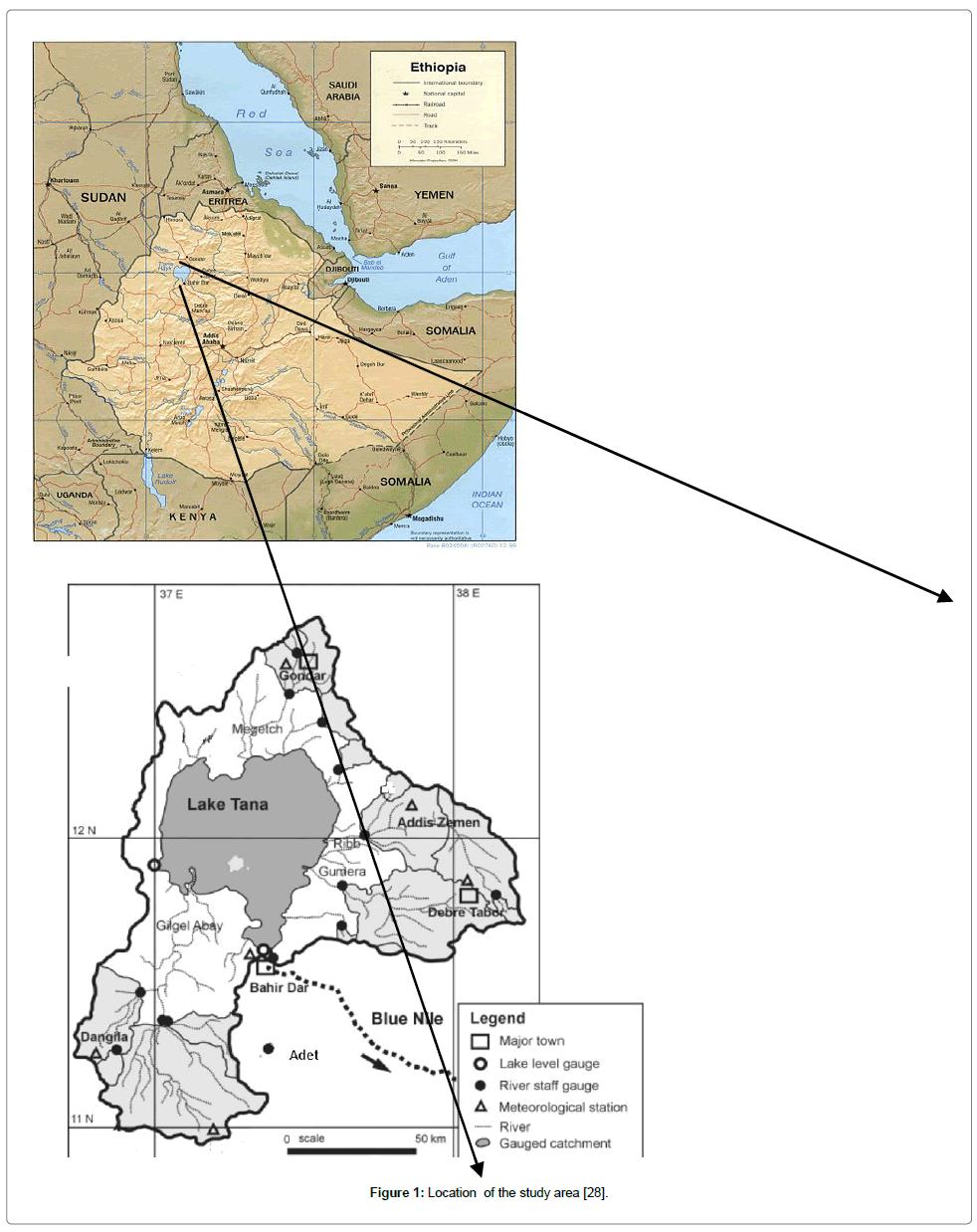
Figure 1: Location of the study area [28].
Conceptual frame work of the study
This study examines the impact of climate change on hydrological drought in the Lake Tana basin. The HBV rainfall-runoff model [26] was used to simulate time series of hydrological data for the drought analyses. Droughts will be identified using the threshold level method [27]. The impact of climate change on hydrological drought for two future periods and one emission scenario, i.e., 2021-2050 and 2071- 2100 under A2 was studied by considering 1971-2000 as a control period.The climate projections were feed into the calibrated HBV model to simulate runoff and then impact of climate change on hydrological drought was assessed. The following shematic diagram (Figure 2) shows the steps followed in this study to assess the impact of climate change on hydrological drought. In the firststep, trend analysis was done for observed hydrometeorlogical data (Boxes 1 and 2). In the Second step, the HBV model was calibrated and validated with local forcing data, streamflow droughts were identified for the validation and calibration periods. The droughts simulated by HBV using local forcing data were compared withdroughts in the observed streamflow data (Box 4). In the third step, recalibration of HBV model was done for the whole observed historical (Box 5) period, for which data is availibile for each sub-basin, droughts were also analysed for this period (Box 4). In the fourth step, recalibratation was again done by forcing HBV with climate data from three GCMs (CNCM3, ECHAM and IPSL) for the historical period (Box 6), then the streamflow droughts derived from the GCMs were compared with droughts obtained in theStep three (Box 7). In the next steps, streamflow was simulated by forcing HBV with three GCMs and using the optimized parameter obtained in Step 4 for three time windows separately; control period (1971-2000) (Box 8), intermediate period (2021-2051) (Box 9).and far future (2071-2100)(Box 10). Finally climate change impact assessment was done by comparing drought chartersitcs drived from GCMs for two future period with droughs in the control period.
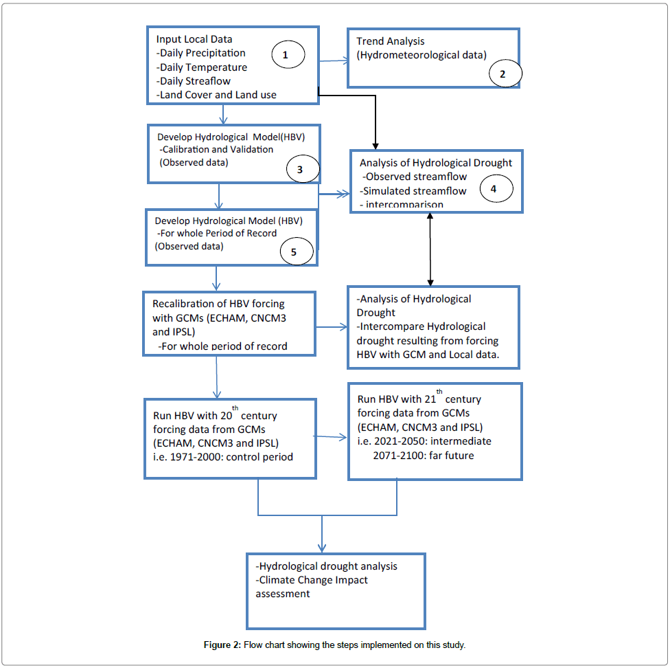
Figure 2: Flow chart showing the steps implemented on this study.
HBV model
Model description: The application of comprehensive physicallybased models is practically not feasible in the study area, because of their high data demand. Instead conceptual hydrological models are preferred as they demand less input (parameters, boundary conditions). HBV model application in scientific research has been reported from more than 50 countries around the world [28]. The HBV model has also been used by different researchers in Ethiopia to model hydrology of basins and to assess the impact the potential impact of climate change [10,28]. The HBV model is a transient, conceptual, semi-distributed hydrological model for simulation of rainfall-runoff relations. It was originally developed at the Swedish Meteorological and Hydrological Institute (SMHI) in the early 70’s to assist hydropower operations by providing hydrological forecasts [29]. The model consists of subroutines for snow accumulation and melt, a soil procedure, routines for runoff generation and a simple routing procedure (Figure 3). The model has been applied in modified versions in many different countries. One of this is the ‘HBV- light’ [26] that provides user-friendly Windows-version for research and education. The HBV-light version provides two options, which do not exist in the HBV-6 version: i) the possibility to include observed groundwater levels into the analysis, and ii) the possibility to use a different response routine with a delay parameter. Calibration of the HBV model was performed by the GAP optimization, using parameter ranges proposed by Seibert et al. [26]. The GAP optimization uses a generic algorism to generate parameter sets that are optimized within the given ranges. The HBV can be used as a semi-distributed model by dividing the basin into sub-basins. Each sub-basin is then divided into zones according to altitude, lake area and vegetation. The HBV model includes a conceptual numerical description of hydrological processes at a basin scale. The general water balance can be described as:
 (1)
(1)
Where: P= precipitation (mm/day), E = evapotranspiration (mm/ day), Q = runoff (mm/day), SP = snow pack (mm), SM = soil moisture (mm), SUZ = upper groundwater zone storage (mm), SLZ = lower groundwater zone storage (mm).
Model calibration and validation: Due to the absence of directly measured basin characteristics, natural variability and non-linearity of the processes involved, calibration of HBV is necessary to adjust the model parameters to improve the model’s ability to reproduce the observed hydrological data (groundwater, streamflow). Input data for calibration and validation of the HBV model are daily values of precipitation, air temperature and potential evapotranspiration for a representative station of the basin.The daily potential evapotranspiration was estimated by the Hargreaves method. For calibration and validation observed streamflow data were collected. The objective of calibration rainfall-runoff models is to optimize parameter sets to match simulated streamflow to observed streamflow [30]. Different ways can be used to assess the fit of simulated streamflow to observed streamflow: e g. visual inspection of plots with Qsim and Qobs, accumulated difference and statistical criteria. The coefficient of efficiency or the Nash- Sutcliffe (NS) efficiency criteria Reffis often used for assessment of simulations by the HBV model [26]. In this study, to give more weight to low flows, the logarithm of Nash-Sutcliffe efficiency (lnReff) was used to evaluate agreement between simulated and observed streamflow.
 (2)
(2)
Where Qsim (mm/day) is simulated flow, Qobs (mm/day) is observed flow, Qobs (mm/day) is the average of observed flow, iis the time step, n is the total number of time steps used during calibration. Nash- Sutcliffe efficiency (NS) can range between −∞ to 1. Reff=1 reflects perfect fit, whereas Reff=0 shows simulations as good (or poor) as a constant-value prediction, and Reff<0 represents very poor fit. NS values between 0.6 and 0.8 indicate fair to good performance and amodel is often said to be perform very good when values are in between 0.8 and 0.9 [30]. The HBV model was calibrated and validated against observed daily streamflow data for each sub-basin and for the whole basin. Calibration was done for both the standard and delay version of HBV model. The period of record for observed streamflow data is different for each sub-basin and therefore the length of periods considered for calibration and validation of the HBV model varies from one basin to another (Table 1). For each of the sub-basins optimized parameter sets were calculated. For optimization of the HBV model parameters, the number of runs was set to 3000 with 50 parameter sets. The number of population was set to with one objective function, Reff (lnReff) which gives more emphasize to low flows. We recalibrated HBV model again using the whole historical data recorded (calibration and validation period) to get a more reliable streamflow simulation. Calibration of HBV model was also made for the three GCMs. for same years as the whole historical record of streamflow data.Then streamflow drought characteristics derived from simulated streamflow with local forcing were compared with the characteristics derived from HBV forced with three downscaled and bias-corrected GCMs (CNCM3, ECHAM and IPSL). The parameters optimized and obtained from calibration of HBV model were used to simulate streamflow for three time windows; control period (1971-2000), intermediate future (2021-2050) and far future or end of the 21st century (2071-2100). Simulation of streamflow was made separately for each time windows (i.e. simulation was not made once for the whole period, 1970-2100). This was done for four sub-basins and for the whole Lake Tana basin. Figure 3 describes the time periods for which the HBV model was run. Then drought analysis was done for each separate period: i.e. calibration period, validation period, whole historical records (calibration + validation), control period (1971-2000), intermediate period (2021-2050) and far future (2071-2100).
| Basin | Calibration Period | Validation Period |
|---|---|---|
| Lake Tana | 1981-1993 | 1994-1998 |
| Gilgel Abbay | 1974-1994 | 1995-2005 |
| Gummera | 1974-1994 | 1995-2005 |
| Ribb | 1981-1997 | 1998-2006 |
| Megech | 1981-1994 | 1995-1998 |
Table 1: Calibration and validation periods.
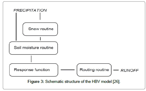
Figure 3: Schematic structure of the HBV model [26].
Data
Observed meteorological and hydrological data: The HBV model simulates daily streamflow using daily rainfall, temperature and potential evaporation as input. The daily precipitation, maximum and minimum temperatures, were obtained from National Meteorological Agency of Ethiopia. The Ministry of Water and Energy collects hydrological data from streams and lake gauging stations. Daily discharge data and lake level were acquired from the Ministry of Water and Energy. Figure 4 provides the climatology of precipitation for the Lake Tana basin. Tables 2 and 3 give an overview of the meteorological and hydrological dataset in the basin for different time periods. Missing data for all hydrometeorological variables was filled by calculating long daily mean for each variable.
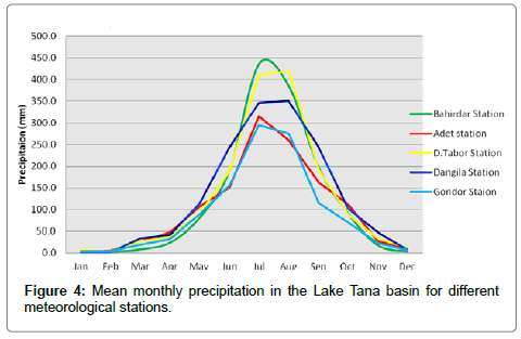
Figure 4: Mean monthly precipitation in the Lake Tana basin for different meteorological stations.
| Station name | Lat. | Lon. | Elevation m amsl | Precipitation | Temperature | |||
|---|---|---|---|---|---|---|---|---|
| Start year | End year | Start year | End year | % of missed data | ||||
| Bahir Dar | 11°36’N | 37°23°E | 1828 | 1961 | 2005 | 1961 | 2005 | 2.4 |
| Gondar | 12°38’N | 37°29’E | 2074 | 1952 | 2007 | 1952 | 2007 | 4.6 |
| Dangila | 11°12’N | 36°52’E | 2126 | 1954 | 2006 | 1954 | 2005 | 5.3 |
| Debre Tabor | 11°50’N | 38°05’E | 2714 | 1951 | 2007 | 1951 | 2006 | 1.7 |
| Adet | 11°16’N | 37°29’E | 2216 | 1986 | 2007 | 1986 | 2005 | 3.8 |
| Addis Zemen | 12°07’N | 37°47’E | 1975 | 1980 | 2006 | 1990 | 2006 | 4.2 |
Table 2: List of meteorological stations used for this study in Lake Tana basin.
| Basins | Lat. | Lon. | Area(km2) | Instantaneous daily flow | ||
|---|---|---|---|---|---|---|
| Start year | End year | % of missed data | ||||
| Lake Tana | 11°35N | 37°24°E | 15046 | 1973 | 2007 | 1.6 |
| Gilgel Abbay | 11°22N | 37°02’E | 1656.2 | 1960 | 2007 | 1.5 |
| Gummara | 11°50N | 37°38’E | 1283.4 | 1960 | 2006 | 2.8 |
| Megech | 12°29N | 37°27’E | 513.5 | 1980 | 2007 | 1.0 |
| Ribb | 12°00N | 37°43’E | 1302.6 | 1961 | 2008 | 4.4 |
| Lake Tana level | 11°36N | 37°23’E | 3060 | 1966 | 2008 | 3.7 |
Table 3: List of gauging stations and lake level used for this study in Lake Tana basin.
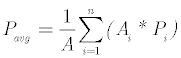
Areal Average precipitation: Areal average precipitation was computed using the Thiessen polygons (Figure 5). This method allocates weight to the station data in proportion of the area of influence that station has. The daily areal average precipitation for the whole basin was calculated from daily point measurement of precipitation of six stations as follows;
 (3)
(3)
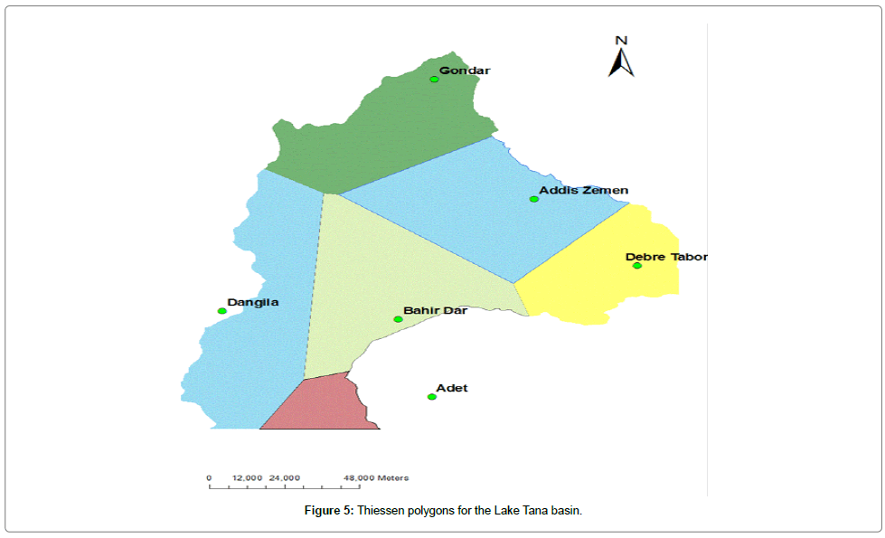
Figure 5: Thiessen polygons for the Lake Tana basin.
Where: Pavg (mm/day) is a real average precipitation, Pi (mm/day) is measured precipitation at station i, i A (km2) is area of influence of subbasin i and A (km2) is the total area of the basin.
Potential evaptransiparation: For stations with limited weather data, like the in this study, the potential evapotransiparation can be calulated in several ways such as the Penman-Montheith equation applied for a refererence crop [31] or Hargreaves et al. [32]. For stations with only temprature but not other variables required by Penman-Montheith equation like sunshine/radation, wind, temprature, humidity, the Hargreaves method can be used to calculate potential evapotransiparation. Hargreaves et al. [32] derived an equation to calculate potential evapotranspiration using only temperature, which is a measurement that can be made most accurately, and extraterrestrial radiation Ra using the relation:
 (4)
(4)
Where : PETHG is the potential evapotransiparation by the Hargreaves method (mm/day), Ra is the extraterresterial radiation (mm/day); Tmean is the averaage tempraure (°C); Tmax and Tmin are the maximum and minimum temprature (°C), respectively.
Future forcing data: General Circulation Models (GCMs) are numerical models, being the most advanced tools currently representing physical processes in the atmosphere, ocean, cryosphere and land surface for simulating the response of the global climate system to increase greenhouse gas concentrations. GCMs depict the climate using a three dimensional grid over the globe, with coarse resolution, typically having a resolution of between 250 km and 600 km horizontally [1].
Global Circulation Models are the best available tools to estimate future global climate changes resulting from the increase of greenhouse gas concentration in the atmosphere [33,34]. However, due to their coarse spatial resolution and associated process description, the outputs from these models may not be used directly in impact studies. Hydrological models that are used for impact studies, for instance, deal with small or sub- basin scale processes whereas GCMs simulate planetary scale and parameterize many regional and smaller-scale processes. Therefore there is a scale mismatch between GCMs and hydrological models and this need downscaling of GCM outputs to basin scale. In this study, downscaled and bias-corrected daily temperature and precipitation data derived from three Atmosphere-Ocean General Circulation Models; ECHAM, IPSL and CNRM (Table 4) from EUWATCH dataset were employed to force the HBV hydrological model for A2 emission scenario. A time slice approach consisting of three time windows with a 30 year period representing historic conditions (control period: 1971-2000) intermediate future (2021-2050) and far future (2071-2100), was adopted for the impact assessment. The GCMs outcome has been downscaled and bias–corrected using the Water and Global Change (WATCH) Forcing Data created for the period 1958-2001 [35]. The WATCH Forcing Data (WFD) is based on the 40 years re-analysis of the European Centre for Medium-Range-Weather Forecast [36]. Weedon et al. [35], interpolated the ERA40 data were to 0.5° and only considered land points using the land-sea mask from the Climate Research Unit dataset TS2.1 [37]. The WATCH future forcing data consist regularly gridded time series of meteorological data (such as rainfall, temperature, snow melt, surface pressure, specific humidity, wind, etc.) with a resolution of 0.5°×0.5° based on sub-daily and daily bases. Daily data were used in this study to force HBV model and to simulate streamflow.
| General Circulation Models (GCMs) | Centre /country | Resolution | |
|---|---|---|---|
| Horizontal | Vertical (layers) | ||
| ECHAM5/MPIOM | MPI-M (Germany) | 1T63 (ca.200 km) | 2L31 |
| CNRM-CM3 | CNRM (France) | T42 (ca. 300 km) | L45 |
| LMDZ-4 | IPSL (France) | T42 (ca.300 km) | L19 |
Table 4: General summary of the General Circulation Models (GCMs) used in this study.
Drought identification
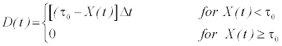
In this study the threshold method [27] was used to detect and analyze hydrological droughts (ground water and streamflow) in the Lake Tana basin. Hisdal et al. [38] distinguished two main approaches for deriving low streamflow and drought characteristics. One approach is to analyze low flow characteristics, such as a time series of the annual minimum n-day discharge, the mean annual minimum n-day discharge or percentile from the flow duration curve (FDC). In the second approach (i.e threshold method), discharge is viewed as a time dependent process and the task is to identify the complete drought event from its first day to the last. In this way a series of drought events can be derived from the discharge series, and drought can be described and quantified by several properties such as drought duration or deficit volume. The threshold approach is the most frequently applied quantitative method, where it is essential to define the beginning and the end of a drought at a site. It is based on defining a threshold, Qo, below which the precipitation, recharge or river flow is considered as a drought. The threshold level method, which generally studies runs below or above a given threshold, was originally named ‘method of crossing theory’ and it is also referred as run–sum analysis [38,39]. The threshold level method originates from the theory of runs introduced by Yevjevich et al. [27], and defines streamflow droughts as periods during which the flow is below a certain threshold level. This method simultaneously characterizes streamflow droughts in terms of duration and deficit volume [40]. Drought events are identified by the threshold level method by first defining a threshold Qx, when the flow is below the threshold value a drought event starts and when the flow equals or rises above the threshold, drought event ends (Figure 6). Then drought characteristics such as onset and end (date), duration (d1, d2,…dn), deficit volume and intensity are identified. The deficit volume in a flux for a particular time step can be calculated from:
 (5)
(5)
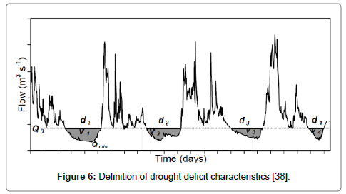
Figure 6: Definition of drought deficit characteristics [38].
Where: D (t) is deficit volume for time step t (L), X(t) is flux for time step t (LT-1), τ0 is threshold (LT-1), and Δt is the time step length (T) A threshold can be fixed or variable. A threshold is regarded as fixed if a constant value is used for the whole series. A variable threshold is a threshold that varies over the year [38]. The threshold level is derived from the flow duration curve. In contrast to flood analysis where non-exceedance values are used, in drought analysis the exceedance value is used, i.e. the value that is equaled or exceeded x% of the time. The threshold might be chosen in a number of ways. For perennial rivers relatively low threshold in the range from Q70 to Q90 can be reasonable [7]. Both the fixed and variable were used in this study. For fixed threshold level the Q80 was used, which is the streamflow value which is equaled or exceeded 80% of the time. For variable threshold, the monthly threshold derived from the 80th percentile of the monthly duration curve smoothed by 30 day moving average was used for drought identification [41]. The variable threshold calculated for the control period was used to identify droughts for the two future periods (Figure 3). When a daily streamflow record is used for drought analysis, besides obtaining a minor drought, several droughts could be obtained which is only a short time apart from each other (mutually dependent droughts) during a prolonged period of drought occurrence [42]. When droughts that are mutually dependent occur a consistent drought definition should include some kind of pooling in order to define an independent sequence of droughts, the pooling procedure removes minor droughts besides pooling mutual dependent droughts [40]. Different pooling procedure available for pooling of mutually dependent droughts and to exclude minor drought are discussed in [40]. The moving average (MA) is the onewhich most effectively removes minor droughts at the same time as it pools dependentdroughts. A MA-filter smooth the original series, since the filtered discharge value for oneday is calculated as average from the n days before and after it [42]. In this study, the 10 days moving average was employed for pooling of mutually dependent droughts and to exclude minor droughts.
HBV model calibration and validation
The HBV model was calibrated and validated against observed daily streamflow data for each sub-basin and for the whole basin. Calibration was done for both the standard and delay version of HBV model. It was found that the HBV using the delay response routine performed well for all sub-basins.Hence results discussed in this report are based on calibration of HBV using the delay response routine. For each of the sub-basins optimized parameter sets were calculated. Table 5 shows the optimized parameter values for each sub-basin and for the whole basin. The logarithmic model efficiency [43], shows the performance of the model which was obtained for calibration and validation periods (Table 6). Rather high values were obtained for all sub-basins. The model efficiency for all sub-basins is above 0.7 for calibration periods and above 0.6 for validation periods. Hence the model performance was assumed to be satisfactory to proceed with the modeling procedure for all sub-basins. We obtained higher NS coefficient for the calibration period for all sub-basins than the ones for the validation period. Although difficult to compare NS values across sub-basins, as different periods of time of record and different number of years were used for calibration and validation, we obtained relatively highest calibration and validation values of NS for GilgelAbbay of 0.90 and 0.81 respectively. Figures 7 and 8 shows the hydrographs of simulated and observed streamflow for the GilgelAbbay River for the calibration and validation periods, respectively. Despite the fact that, the HBV model does not reproduce the high flow very well, there is a high agreement between the observed and simulated streamflow for intermediate and low flows, which we particularly focus in this study. A visual inspection of observed and simulated streamflow for both the calibration and validation periods reveals that, the hydrograph of the observed flow exhibits higher fluctuation. The hydrograph of the simulated streamflow is more smooth and regular. The flow duration curve (FDC) was also computed to see how the observed and simulated streamflow matches. Figures 9 and 10 are the flow duration curve for the calibration and validation period respectively. From the Figures we can deduce that for low flow the observed and simulated streamflow curves are close to each other, however, as the streamflow increase the FDC curves deviates. The rather large difference between observed and simulated flow in high flow is due to the fact that the HBV model was calibrated with ln Reff, which give more emphasis to low flow.
| Parameters | Lake Tana | G.Abbay | Gumara | Ribb | Megech |
|---|---|---|---|---|---|
| FC | 709 to 879 | 119 to 187 | 335 to 396 | 135 to 751 | 280 to 413 |
| LP | 0.20 to 0.29 | 0.99 | 0.64 to 0.99 | 0.33 to 0.78 | 0.31 to 0.37 |
| BETA | 4.1 to 6.8 | 1 | 1 to 4.67 | 1.16 to 4.2 | 1.69 to 7 |
| Delay | 0.999 | 0.53 | 10.69 | 3.41 | 2 |
| Alpha | 0.38 | 0.61 | 0.69 | 1.2 | 1.04 |
| PART(-) | 0.96 | 0.96 | 0.99 | 0.99 | 0.99 |
| K1 | 0.0029 | 0.0034 | 0.0022 | 0.0036 | 0.0036 |
| K2 | 0.0068 | 0.0005 | 0.0022 | 0.0024 | 0.00084 |
| MAXBAS | 13.9 | 2 | 2 | 2.38 | 2 |
Table 5: Optimized model parameter each sub-basins (range for difference vegetation zones).
| Basins/sub-basins | Nash-Sutcliffe effeciency | |
|---|---|---|
| Calibration | Validation | |
| Lake Tana | 0.85 | 0.60 |
| Gilgel Abbay | 0.90 | 0.81 |
| Gummera | 0.89 | 0.61 |
| Megech | 0.8 | 0.71 |
| Ribb | 0.73 | 0.68 |
Table 6: The Nash-Sutcliffe logarithmic model efficiency for different sub-basins and the whole Lake Tana basin.
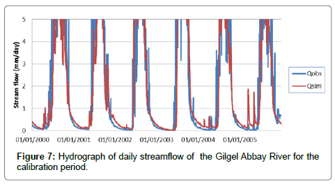
Figure 7: Hydrograph of daily streamflow of the Gilgel Abbay River for the calibration period.
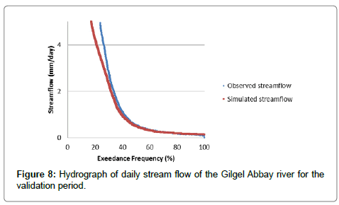
Figure 8: Hydrograph of daily stream flow of the Gilgel Abbay river for the validation period.
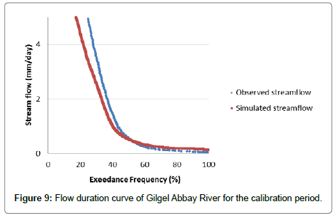
Figure 9: Flow duration curve of Gilgel Abbay River for the calibration period.

Figure 10: Flow duration curve of Gilgel Abbay River for the validation period.
Changes in future hydrometeorological variables
Precipitation: Figures 7 show the changes in mean monthly precipitation as simulated by CNCM3, ECHAM and IPSL, respectively. The change in precipitation does not reveal a clear trend for all GCMs and for both future periods. The change varies per month. For example, for the main rainy season JJAS (June, July, August and September), according to CNCM3, June precipitation increases by 15 and 17% for the period 2021-2050 and 2071-2100, respectively (Figure 11). Precipitation shows a small reduction in July, August and September. Precipitation shows a small increase for the other months like October, November and December. For example, October precipitation changes by 63 and 83% for 2021-2050 and 2071-2100 respectively. In November these numbers are 10 and by 155%. A huge change is projected by CNCM3 for December, the precipitation increases by 127% and 240%, although change in absolute precipitation is relatively small (0.25-0.6 mm/d). ECHAM projects decreasing trends for months January to June and decreasing trends for months July to December (Figure 12). Unlike the change in precipitation according to CNCM3 in June, ECHAM precipitation decreases by 28 and 43% for the two future periods 2021- 2050 and 2071-2100, respectively. There is a significant increase in precipitation on August, September and October by 16, 46 and 145% in the year 2071-2100, respectively. The pattern of change in precipitation projected by ISPL is different from both CNCM3 and ECHAM for most months of the year (Figure 13). There is a small increase in precipitation in January, February, March and December for both future periods. A significant decrease in precipitation is experienced on June, precipitation decreases by 20 and 21% for 2021-2050 and 2071- 2100 respectively. Increasing trends in precipitation are observed for July, August and September. Precipitation increases by about 45 and 33% respectively, in September. In summary for the summer season, (JJAS) in which the basin receives above 70% of the rainfall amount, the precipitation increased by about 2.6 and 5.7% for ECHAM and IPSL, respectively, while CNCM3 predicts a reduction in precipitation by about 5.8% for the intermediate future. At the end of the 21st century ECHAM and IPSL project again an increase in precipitation by about 3.5 and 5.8% respectively, while CNCM3 projects a small reduction by 0.3%. As a summary, though there are no clear trends in change in precipitation, for winter months, the precipitation shows an increasing trend. While the precipitation changes by small amount or show a significant decrease in some of the summer months like June when the basin receives more than 70% of the total precipitation. The significant increase in winter precipitation for both future periods could indicate that there would be also seasonal shift in precipitation due to the changing climate.
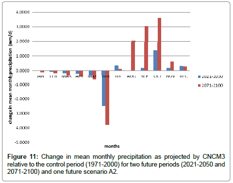
Figure 11: Change in mean monthly precipitation as projected by CNCM3 relative to the control period (1971-2000) for two future periods (2021-2050 and 2071-2100) and one future scenario A2.
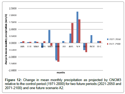
Figure 12: Change in mean monthly precipitation as projected by CNCM3 relative to the control period (1971-2000) for two future periods (2021-2050 and 2071-2100) and one future scenario A2.
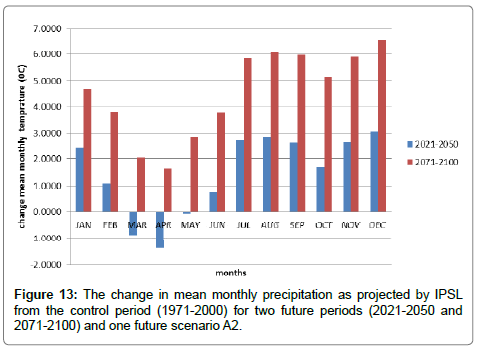
Figure 13: The change in mean monthly precipitation as projected by IPSL from the control period (1971-2000) for two future periods (2021-2050 and 2071-2100) and one future scenario A2.
Temperature: Unlike precipitation, the mean temperature shows clear increasing trends for almost all months of the year and for both periods. Figure 14 shows change in mean monthly temperature for CNCM3 two future periods relative to the control period. The maximum change in mean temperature for the intermediate period is expected on December. The temperature increases by about 3°C for this month. At the end of the 21st century (2071-2100) an increase in mean temperature is projected in all months of the year. The minimum increase in mean temperatures is projected in April which is 1.7°C and the maximum increase in mean temperature is projected in December, which is 6.5°C. For the intermediate future (2021-2050) decreasing trends are detected, in March and April. The mean temperature decreases then by 0.9 and 1.4°C, respectively. Figures 15 and 16 depict changes in mean temperature for two future periods for as simulated by ECHAM and ISPL, respectively relative to the control period (1971-2000). The change in mean temperature for ECHAM varies per month for intermediate future. Mean temperature decrease on April and May by about 0.23 and 0.13 respectively. For the other months of year, temperature is projected to increases from a minimum of 0.01°C in January to 1.8°C in December. At the end of the 21st century mean temperature is expected to increase for all months of the year. The minimum and maximum mean temperature increases are projected on January and September respectively. The minimum and maximum changes projected are about 2.5 and 4.5°C respectively.In summary, all models project that the mean temperature will increase in most months of the year for the intermediate future period. For this period the maximum increase is projected by CNCM3, about 3°C. Model projections agree that the mean temperature will increase significantly at the end of the 21st century. The minimum increase in mean monthly temperature for this period is projected by CNCM3, about 1.7°C and the maximum is projected by ISPL, about 8.9°C.
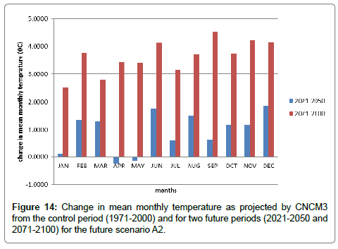
Figure 14: Change in mean monthly temperature as projected by CNCM3 from the control period (1971-2000) and for two future periods (2021-2050 and 2071-2100) for the future scenario A2.
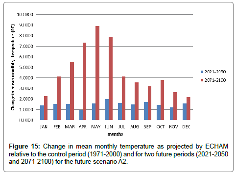
Figure 15: Change in mean monthly temperature as projected by ECHAM relative to the control period (1971-2000) and for two future periods (2021-2050 and 2071-2100) for the future scenario A2.
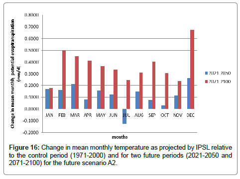
Figure 16: Change in mean monthly temperature as projected by IPSL relative to the control period (1971-2000) and for two future periods (2021-2050 and 2071-2100) for the future scenario A2.
Potential evapotranspiration: Potential evapotranspiration depends among others on the basin temperature. Thus potential evapotranspiration will also be affected by the climate change impacts on temperature. In this study the potential evapotranspiration is calculated with the Hargreaves’ approach. Figure 17 shows the change in mean monthly potential evapotranspiration period for CNCM3 and for two future periods with respect to the control period. The potential evapotranspiration is projected to increase for all months of the years, except July for the intermediate future period. For this month the potential evapotranspiration is expected to decrease by 2.6%. The minimum and maximum increase in potential evapotranspiration is expected in October and December by 0.6 and 6.2% respectively. At the end of the 21st century potential evapotranspiration is projected to increase in all months of the year. The minimum and maximum increase in potential evapotranspiration is 3.9% and 15% in January and December respectively.For ECHAM the potential evapotranspiration is projected to decrease in April and May by 6 and 1%, respectively for the intermediate period (Figure 18). The potential evapotranspiration increase for the other months of the year in this period. The minimum increase in evapotranspiration is expected in January (0.2%) and the maximum increase in potential evapotranspiration is expected in June (8.9%). At the end of 21st century potential evapotranspiration is projected to increase in all months of the year. Figure 19 depicts the change in mean monthly potential evapotranspiration for IPSL relative to the control period. A decrease has been projected for most of the months of the year for the intermediate period. At the end of the 21st, the potential evapotranspiration is expected to increase in all months of the year except, April. The maximum increase is expected in June. In this month the potential evapotranspiration is projected to change by about 11.4%. In summary, for the summer season (JJAS), the potential evapotranspiration, which is calculated by Hargreaves’s equation, is projected to increase in most months according to CNCM3 and ECHAM for both future periods, while IPSL does not show a clear trend. For the summer season, the change in potential evapotranspiration is projected to increase in both intermediate and far future for all GCMs. The change is projected to be 1.2, 4 and 2% for CNCM3, ECHAM and IPSL, respectively, in the intermediate future. At the end of the 21st century the change in potential evapotranspiration is projected to be even higher, namely 5.7, 10.7 and 4.2% for CNCM3, ECHAM and IPSL, respectively.
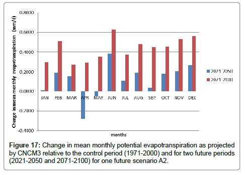
Figure 17: Change in mean monthly potential evapotranspiration as projected by CNCM3 relative to the control period (1971-2000) and for two future periods (2021-2050 and 2071-2100) for one future scenario A2.
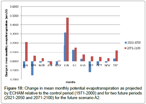
Figure 18: Change in mean monthly potential evapotranspiration as projected by ECHAM relative to the control period (1971-2000) and for two future periods (2021-2050 and 2071-2100) for the future scenario A2.
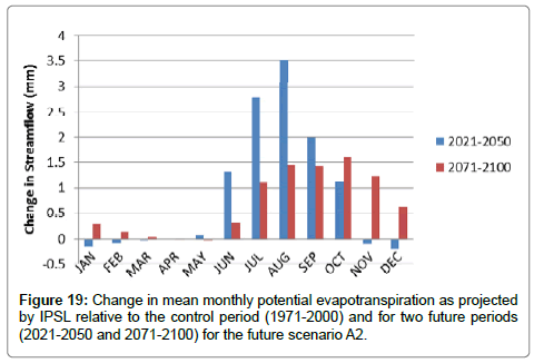
Figure 19: Change in mean monthly potential evapotranspiration as projected by IPSL relative to the control period (1971-2000) and for two future periods (2021-2050 and 2071-2100) for the future scenario A2.
Streamflow: HBV using forcing of the CNCM3 model projected an increase in streamflow for both the intermediate and far future periods in most of the months of the year as depicted in Figure 20. The projected increase in the streamflow is especially significant during the main rainy season (June-September). According to ECHAM model forcing, the streamflow is projected to increase in all months of the year for the intermediate future (Figure 21). For the far future the streamflow is also projected to increase for all months, except August. For ECHAM model the projected increase in streamflow is small in the main rainy season compared to other seasons which are opposite to CNCM3. While both the CNCM3 and ECHAM forcing of HBV projected an increase in streamflow in the main rainy season, IPSL projected a significant decrease in the main rainy season (Figure 22) for the intermediate and far future periods. A significant increase is projected by IPSL in the dry months where no/small amount of rain is expected, such as January to April (Figure 7).
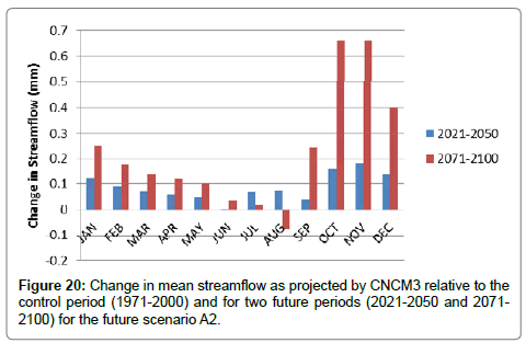
Figure 20: Change in mean streamflow as projected by CNCM3 relative to the control period (1971-2000) and for two future periods (2021-2050 and 2071- 2100) for the future scenario A2.
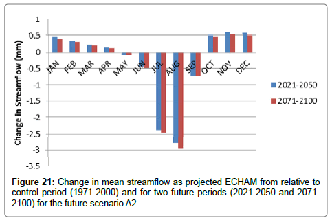
Figure 21: Change in mean streamflow as projected ECHAM from relative to control period (1971-2000) and for two future periods (2021-2050 and 2071- 2100) for the future scenario A2.
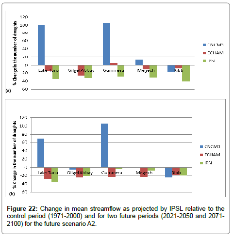
Figure 22: Change in mean streamflow as projected by IPSL relative to the control period (1971-2000) and for two future periods (2021-2050 and 2071- 2100) for the future scenario A2.
Drought characteristics for future periods
To quantify the impact of climate change on streamflow drought characteristics, the percentage change of streamflow drought characteristics was calculated using GCM forcing (ECHAM, CNCM3 and IPSL) for two future periods relative to the control period. Figure 23 depicts the percentage change of the number streamflow drought for the intermediate future and end of the 21st century for each whole Lake Tana basin and sub-basin. When we consider the number of drought in the Lake Tana basin, more droughts are expected for both the intermediate and far future according to CNCM3, while for the ECHAM and IPSL forcing a decrease in number of droughts for both future periods is projected. According to CNCM3, the number of droughts in the Lake Tana basin is expected to increase by 100 and 68.8% in the intermediate and far future, respectively. IPSL projected a decrease in the number of streamflow drought by 35% for the intermediate and far future. ECHAM also projected a decrease in the number of streamflow drought by 16 and 28% for intermediate and far future, respectively. According to IPSL the number of droughts are projected decrease for all sub-basins and ECHAM also projected a decrease in the in the number of droughts for all sub-basins except Gummera for intermediate future. For Gummera, ECHAM projected an increase in the number of droughts. For the far future, both IPSL and ECHAM projected a decrease in all sub-basins for the far future. Generally, no clear patterns (direction and magnitude) can be observed on how the projected climate change would impact on the number of streamflow droughts in the Lake Tana basin, in general and in each sub-basin, except for the Ribb and GilgelAbbay sub-basins. In the Rib sub-basin all GCMs agree on a decrease of the number of droughts for both intermediate and far future by 10-40%. In GilgelAbbay subbasin all GCMs also projected a decrease in the number of droughts. Figure 24 depicts change in average drought duration (%) projected by HBV using the forcing from three GCMs relative to the control period for the intermediate and far future (end of the 21st century). According to IPSL forcing, the average drought duration for the Lake Tana basin is likely to increase significantly for both the intermediate and far future. In contrast, the average drought duration is projected to decrease in the intermediate and far future periods for both CNCM3 and ECHAM forcings. For example, for the Lake Tana basin, IPSL projected an increase in the average drought duration by 80 and 95% for the intermediate and far future respectively. CNCM3 projected a decrease in average drought duration by 36 and 48%, and ECHAM a reduction by 42 and 21%, respectively. According to IPSL forcing, average drought duration is projected to reduce in all sub-basins for both intermediate and far future. For ECHAM, the average drought duration is expected to decrease in all sub-basins except GilgelAbbay for intermediate future. For far future the ECHAM forcing projected an increase for all sub-basins. For the Lake Tana basin, the average deficit volume is projected to reduce in the intermediate period for HBV using CNCM3 and ECHAM forcing by about 20 and 3% respectively (Figure 25). At the end of the 21st century, the deficit volume is also projected to decrease by about 33 and 2% for CNCM3 and ECHAM forcing respectively. For the IPSL forcing, the deficit volume is expected to increase by 9 and 19% respectively, for the intermediate and far future periods. According to the CNCM3 and ECHAM forcing, for all sub-basins the average deficit volume is projected to increase for both intermediate and future periods. All models agree on the direction of projection of average deficit volume for Megech and Ribb sub-basins for intermediate period (Figure 25). For far future the three models agree on three sub-basins on projection of average deficit volume. In summary, HBV forcing using two GCM forcing (ECHAM and IPSL) out of three (except ECHAM in the Gummer sub-basin), agree in the direction of change in the number of droughts for the intermediate and far future. In both models the number of drought expected to reduce in intermediate and far future periods. On the contrary, CNCM3 projected a substantial increase in the number of droughts in the Lake Tana basin and Gummer sub-basin in the intermediate and far future periods. Both ECHAM and CNCM3 projected that droughts will sustain for shorter periods, for the intermediate and far future in the Lake Tana basin. According to ISPL, droughts were projected to sustain for shorter time period in all sub-basins for the intermediate period and far future in all sub-basins except the Lake Tana basin. In the Lake Tana basin, two out of three models agree in projecting a small increase in average deficit volume. For all sub-basins, both CNCM3 and ECHAM agree in the direction of change of the average deficit volume for the intermediate and far future. In general, model projection of drought characteristics for future periods do not agree on the direction and magnitude of the drought characteristics for the Lake Tana basin and for all sub-basins. The different results in drought characteristics for the same models across different basins could be attributed to the difference in the hydrological properties, topography, land use and land cover for each sub-basin. And the differences in projection of future drought characteristics among the three models might be due to the structure of the models, model parameterization and also initial condition used in the three different models.
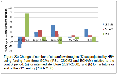
Figure 23: Change of number of streamflow droughts (%) as projected by HBV using forcing from three GCMs (IPSL, CNCM3 and ECHAM) relative to the control period: (a) for intermediate future (2021-2050), and (b) for far future or end of the 21st century (2071-2100).
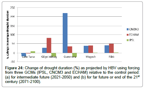
Figure 24: Change of drought duration (%) as projected by HBV using forcing from three GCMs (IPSL, CNCM3 and ECHAM) relative to the control period: (a) for intermediate future (2021-2050) and (b) for far future or end of the 21st century (2071-2100).
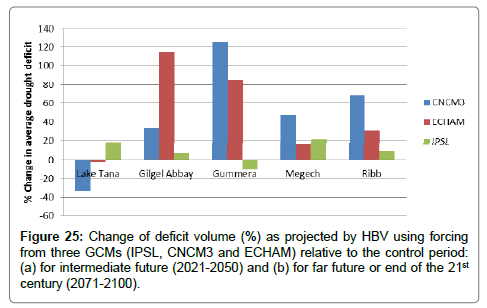
Figure 25: Change of deficit volume (%) as projected by HBV using forcing from three GCMs (IPSL, CNCM3 and ECHAM) relative to the control period: (a) for intermediate future (2021-2050) and (b) for far future or end of the 21st century (2071-2100).
As changes in temperature and precipitation affect streamflow in a basin, it is worthwhile to discuss how the climatic variables are affected due to climate change. Two out of three GCMs projected that, the mean temperature increases in most months of the year for the intermediate future period (2021-2050). For this period the minimum increase in mean monthly temperature is projected by ECHAM (about 0.01°C) and the maximum is projected by CNCM3 (about 3°C). All the model projections agree that the mean monthly temperature will increase significantly at the end of the 21st century. The minimum increase in mean temperature for this period is projected by CNCM3 (about 1.7°C) and the maximum is projected by ISPL (about 8.9°C). In their study on impacts of climate change on Blue Nile flows using 17 GCMs [44] documented that all models predict an increase in annual surface temperature at the end of the 21st century compared to the baseline period with values that ranges from 2 to 5°C. The three GCMs used in this study disagree on the direction of precipitation changes. For intermediate period precipitation changes ranges from -38% in March to 127% in December, from -48% in February to 330% in December, from -30% in April to 79% in January for CNCM3, ECHAM and IPSL respectively. For the far future precipitation changes ranges from -25% in February to 240% in December, from -90% in February to 310 % in December, from -27% in October to 155% in January for CNCM3, ECHAM and IPSL respectively. For the summer season, (JJAS) in which the basin receives above 70 -90% of the total rainfall, the precipitation increased by about 2.6 and 5.7% for ECHAM and IPSL, respectively, while CNCM3 projects a reduction in precipitation by about 5.8% for the intermediate future. At the end of the 21st century both ECHAM and IPSL project an increase in precipitation by about 3.5 and 5.8% respectively, while CNCM3 projects a small reduction by 0.3%. The global distribution of 2080-2099 change in annual mean precipitation for SRES AlB scenario from a 15-model ensemble shows an increase in annual precipitation exceeding 20% occur in most high latitudes, as well as in North Africa and to increase by around +7% in tropical and eastern Africa will be drier [1]. The potential evapotranspiration was generally predicted to increase in most of the months using CNCM3 and ECHAM forcing for both future periods, while for IPSL it does not show a clear trend. For the summer season, the change in potential evapotranspiration is projected to increase in both intermediate and far future for all GCMs. The change is projected to be 1.2, 4 and 2% for CNCM3, ECHAM and IPSL, respectively in the intermediate futures. At the end of the 21st century the change in potential evapotranspiration is projected to be even higher, 5.7, 10.7 and 4.2% for CNCM3, ECHAM and IPSL, respectively. Studies done by Elshamy et al. [44] reported an increase in wet (summer) season potential evapotranspiration varying from 2 to 14%. According to IPCC [1], evapotranspiration demand or potential evaporation is projected to increase almost everywhere. This is because, the water holding capacity of the atmosphere increases with higher temperature but relative humidity is not projected to increase markedly. Table 8 describes the change in direction, magnitude and agreements among GCMs projected for both the intermediate and far future periods for drought characteristics. In the IPCC [1] report,the increase in rainfall in east Africa, extending into the horn of Africa is robust across the ensembles of models, with 18 out of 21 models projecting an increase in the core this region, east of the great lakes. According to CNCM3, the number of droughts is projected to increase for Gummer, Megech and the whole Lake Tana basin for the intermediate period. ECHAM projected a decrease in the number of droughts for all basins except Gummer. IPSL projected a decrease in the number of droughts for all basins. At the end of the 21st century, both IPSL and ECHAM projected a decrease in the number of droughts.But CNCM3 projected an increase in the number of droughts for Gummer and for the whole Lake Tana basins (Table 7). For the intermediate period, the average drought duration is projected to increase in most of the basins according to CNCM3, but both IPSL and ECHAM projected a decrease in most of the basins.For the far future, the average drought duration is projected to increase in most of the basins based on ECHAM and CNCM3. While the average drought duration is projected by IPSL shows a decrease in most of the basins (Table 8). The average deficit volume is projected to decrease in most the basins according to all GCMs for both intermediate and far future periods (Table 9).
| Basin | Intermediate period (2021-2050) | Agreement | Far future (2071-2100) | Agreement | |||||
|---|---|---|---|---|---|---|---|---|---|
| IPSL | ECHAM | CNCMB | IPSL | ECHAM | CNCMB | ||||
| Lake Tana | -- | - | + | 2↑ | -- | - | + | 2↑ | |
| Gilgel Abbay | -- | - | 0 | 2↓ | -- | --- | - | 3↓ | |
| Gummera | - | + | ++ | 2↑ | - | -- | + | 2↓ | |
| Megech | -- | - | + | 2↓ | - | -- | 0 | 2↓ | |
| Ribb | --- | -- | - | 3↓ | - | -- | --- | 3↓ | |
Table 7: The change in direction, magnitude and agreement among GCMs of the number of droughts for the intermediate and far future periods. The + and – signs show the direction of the change in number of droughts and the number of the + and – sign shows the magnitude of the change.
| Basin | Intermediate period (2021-2050) | Agreement | Far future (2071-2100) | Agreement | ||||
|---|---|---|---|---|---|---|---|---|
| IPSL | ECHAM | CNCMB | IPSL | ECHAM | CNCMB | |||
| Lake Tana | + | -- | - | 2↓ | + | - | - | 2↓ |
| Gilgel Abbay | - | ++ | + | 2↑ | - | ++ | + | 2↑ |
| Gummera | - | - | + | 2↓ | - | + | ++ | 2↑ |
| Megech | -- | - | - | 3↓ | - | + | - | 2↓ |
| Ribb | -- | - | + | 2↓ | - | + | ++ | 2↑ |
Table 8: The change magnitude, direction and agreement among GCMs of the average drought duration for the intermediate and far future periods. The + and – signs show the direction of the change in number of droughts and the number of the + and – sign shows the magnitude of the change.
| Basin | Intermediate period (2021-2050) | Agreement | Far future (2071-2100) | Agreement | |||||
|---|---|---|---|---|---|---|---|---|---|
| IPSL | ECHAM | CNCMB | IPSL | ECHAM | CNCMB | ||||
| Lake Tana | + | - | - | 2↓ | + | - | - | 2↓ | |
| Gilgel Abbay | - | ++ | + | 2↑ | + | +++ | ++ | 3↑ | |
| Gummera | - | + | ++ | 2↑ | - | ++ | +++ | 2↑ | |
| Megech | + | +++ | ++ | 3↑ | ++ | + | +++ | 3↑ | |
| Ribb | + | +++ | ++ | 3↑ | + | ++ | +++ | 3↑ | |
Table 9: The change direction, magnitude and agreement among GCMs of the average drought deficit for the intermediate and far future periods. The + and – signs show the direction of the change in number of droughts and the number of the + and – sign shows the magnitude of the change.
According to IPCC [1], streamflows are likely to be influenced by climate change. The possible range of Africa-side climate change impacts on streamflow is predicted to change significantly between 2050 and 2100, from -15 to +5% above the 1961-1990 baseline in 2050 and rising to -19 to +14% in 2100. Different studies have been undertaken on the impact of climate change on the hydrological resource of the Blue Nile basin in general and Lake Tana basin in particular. Elshamy et al. [44] analyzed the output of 17 GCMs to study the impact of climate change in the Upper Blue Nile Basin where Lake Tana basin is located for 2081-2098 period. There result shows no consensus among the change in direction of total annual precipitation that ranges from -15% to + 14% with more models report reductions than those reporting increase. This difference in projection of precipitation among different GCMs also is manifested in projected drought characteristics in the Lake Tana basin. There is no consensus in the direction and magnitude of change in hydrological drought characteristics from one basin to another for the same GCM (Table 8) which could be due to the relative large variability across sub-basins with respect to climate, topography and physiographical or hydrological characteristics [30]. There is also large difference in the direction and magnitude of change of drought characteristics among GCMs in the same basin or sub-basin. The variation among the GCMs is due to the fact that different climate models have different model structure and hence exhibit a wide range of climate sensitivities [1]. This difference among climate models is a large source of uncertainty, projections becomes less consistent as the spatial scale decreases. Therefore the spread in projected streamflow drought characteristics (Table 8) is an indication of uncertainties in climate change projections among GCMs. Further sources of uncertainty in hydrological projection arise from the structure of the current climate models, i.e. current climate models generally exclude some feedbacks from vegetation change to climate, and many of the simulations used for deriving climate projections also exclude anthropogenic changes in land cover [45]. Another study on the investigation of the impact of climate change on hydrological extremes [12] using 17 GCMs for A1B and B1 scenario on the Lake Tana basin showed a wide range of abilities in simulation rainfall, maximum and minimum temperature, and the result revealed unclear trends for low flows for 2050s. Consistent to this result, the projected hydrological drought characteristics by the three GCMs, varies in the sign and magnitude in the same basin, and across sub-basins. Study done by Taye et al. [12], it is also documented that in annual, seasonal and monthly scale, approximately half of the GCM runs project increased flow and the other half project decreases. Other studies [11,13] on the impact of climate change on the hydrological resources of Lake Tana basin revealed that four of the nine GCMs investigated showed a statistically significant decline in annual streamflow during mid (2040-2069) and late (2070-2099) as a result of both precipitation declines and increase in evaporative demand because of the increase in temperature. For example, by 2070-2099 precipitation projection for the Blue Nile basin range from (-36% to 24% with multimodel median of 24%), resulting in streamflow projections ranging from -29% to 23% with a multimodel median of -10%. According (IPCC, 2007) [1] fourth assessment report, droughts have become longer and more intense, severe, and have affected larger areas since the 1970s; the land area affected by drought is expected to increase and water resources availability in affected areas could decline as much as 30 present by mid-century. More severe droughts are projected in all sub-basins for both periods. The projected change in severity of droughts is less in the Lake Tana basin compared to all sub-basins; this could be due to the large storage of the Lake.
The Lake Tana basin is potentially rich in water. For this case, it has been identified as a development corridor by the government and the World Bank [5]. The basin contains three hydropower plants, which has a very high national importance in meeting the growing energy demand of the country. There are also many irrigations project plans in each of the sub-catchments which are already completed and ongoing.Drought is a common natural phenomenon in the region, which have been imposing food insecurity and other complex problems. Severe droughts happened once every 10 years in the region and now becoming more frequent and covering areas that never experience drought before, in the southern parts of the country. According to IPCC [1] droughts will become more intense, frequent and severe in the future due to the impact of climate change. Therefore it is very essential to assess the impact of climate change on hydrological drought in the Lake Tana basin for effective water management and planning. In this study the impact of climate changes on hydrological drought in the Lake Tana basin in Ethiopia, which is the headwater for the Blue Nile River, was assessed. For this purpose the rainfall-runoff HBV model was calibrated and validated with local historical data to investigate the possible impact of climate change on hydrological drought in the basin for four sub-basins and the Lake Tana basin. Data sets obtained from EU-WATCH projectfor threeGeneral Circulation Models (CNCM3, IPSL and ECHAM) were used as an input to the HBV model to derive future streamflow for two future time windows (2021-2050 and 2071-2100) and for one future emission scenario A2. The threshold level method combined with a 10-day moving average streamflow was used to detect hydrological drought characteristics. The model efficiency obtained for all subbasins is above 0.7 for calibration periods and above 0.6 for validation periods. Hence the model performance is assumed to be satisfactory for all sub-basins. Thus, the HBV model can be used for hydrological modeling and analysis in the Lake Tana basin. Trend analysis was done for the time series of hydrometeorological varibales. No trends were detected in precipitation time series. All station shows an upward trend in maximum temperature for Mann-Kendall trend test, while Gondar and Addis Zeman revealed a downward trend for minimum temperature. Mann-Kendall and Sen Slope trend tests only dis agree on the direction of trend for maximum temperature for Gondar station. Both Mann-Kendall trend test and Sen Slope agree in the direction of trends in streamflow. There is an increasing trend in streamflow in all rivers except GilgelAbbay which shows a decreasing trend. The number of droughts in observed streamflow exceeds the number of droughts in streamflow simulated with HBV using local forcing data in all four sub-basins. The average drought duration and average deficit volume are higher in simulated streamflow in all sub-basins except Lake Tana basin.Intercomparison of drought characteristics simulated with HBV using local forcing’s data with that from GCMs outputs for historical period revealed that all GCMs underestimated the number of droughts in the range -38 to 68% in the Lake Tana basin (Figure 7). Two GCM (CNCM3 and ECHAM) among three estimated the same number of droughts. IPSL underestimated the number of droughts by about 68%. This shows a great difference between the number of droughts using IPSL output and the ones using local forcing data. Both CNCM3 and ECHAM agree in the sign of estimating drought duration. The average drought duration by CNCM3 and ECHAM is overestimated by 47 and 49%, respectively. The deficit volume is over estimated by all GCMs in the Lake Tana basin. CNCM3 and ECHAM agree on the sign of estimating all drought characteristics in the Lake Tana basin. In the intermediate future the minimum increase in mean temperature is projected by ECHAM (about 0.01°C) and the maximum is projected by CNCM3 (about 3°C). While all the model projections agree that the mean temperature will increase significantly at the end of the 21st century. The minimum increase in mean temperature for this period is projected by CNCM3 (about 1.7°C) and the maximum is projected by ISPL (about 8.9°C). For the summer season (JJAS) in which the basin receives above 70-90% of the total rainfall, the precipitation changes by about 2.6 and 5.7% for CNCM3 and IPSL respectively, while ECHAM predicts a reduction in precipitation by about 5.8% for the intermediate future. At the end of the 21st century both ECHAM and IPSL project an increase in precipitation by about 3.5 and 5.8% respectively, while CNCM3 projects a small reduction of 0.3%. For the summer season, the change in potential evapotranspiration is projected to increase in both intermediate and far future for all GCMs. The change is projected to be 1.2, 4 and 2% for CNCM3, ECHAM and IPSL, respectively in the intermediate futures. At the end of the 21st century the change in potential evapotranspiration is projected to be even higher, 5.7, 10.7 and 4.2% for CNCM3, ECHAM and IPSL, respectively.The impact of climate change on hydrological drought characteristics was assessed for two future period; intermediate period (2021-2050) and far future (2071-2100). The percentage change in drought characteristics was computed with respect to the base period (1971-2000). According to HBV using CNCM3 forcing, the number of droughts in the Lake Tana basin is expected to increase by 100% and 68.8% in the intermediate and far future respectively. IPSL projected a decrease in the number of streamflow drought by 35% for the intermediate and far future. ECHAM projected also projected a decrease in the number of streamflow drought by 16 and 28% for intermediate and far future, respectively. On the contrary, IPSL projected an increase in the average drought duration by 80 and 95% for the intermediate and far future, respectively. CNCM3 projected a decrease in average drought duration by 36 and 48% for the intermediate and far future respectively. According to ECHAM the average drought duration in the Lake Tana basin projected to reduce by 42 and 21%, respectively. The average deficit volume is projected to substantially reduce in the intermediate period for CNCM3 and ECHAM by about 20 and 3% respectively. At the end of the 21st century, the deficit volume also projected to decrease by about 33 and 2% for CNCM3 and ECHAM respectively. For the IPSL model, the deficit volume is expected to increase by 9 and 19%, respectively for the intermediate and far future periods. Generally, there is no general consensus among GCMs used in this study towards a distinct change in magnitude and direction in projection of change in the characteristics of streamflow droughts. These uncertainties in projecting the impact of climate change on hydrological drought may arise from several factors. Among these are the formulation and accuracy of the General Circulation Models GCMs), choice of emission scenarios and the hydrological model itself (i.e. HBV). In this study only three GCMs and one emission scenario have been employed. To account for GCM and scenario uncertainties, use of ensembles of GCMs and scenarios is recommended for assessment of climate change impact on hydrological drought. And to account for the uncertainty due to the hydrological model, two or more hydrological models could be used. Uncertainty could also arise from a scale mismatch between GCMs and hydrological models.For a catchment that shows high spatial variability like the Lake Tana basin, Regional Climate Models (RCM) provide climate information with useful local detail including realistic extreme events. Therefore regional climate models (RCMs) that provide the finest resolutions and able to capture small scale atmospheric process and topographic difference in the basin could obtain a better climate change impact assessment on hydrological droughts.