Journal of Research and Development
Open Access
ISSN: 2311-3278
ISSN: 2311-3278
Research Article - (2025)Volume 13, Issue 2
In Doyogena town water drainage system is the main problem of the community in their daily life. However, the drainage situation and the maximum runoff in the area are not estimated. This study aims to assess the drainage condition of the town and thereby estimate the maximum peak discharge using best-fit probability distribution function. Climate data, field survey and secondary data were used for analysis of this study using GIS and remote sensing for driving intensity duration and frequency relations and computing the hydraulic performance of the EDS of the town. The main finding of this study indicated that high problem of water drainage system in Doyogena town due to many long-lived challenges such as lack of enough water flow lines, less focus given to rehabilitate roads and lack of awareness about prevention of dry wastes and so on. Additionally; a researcher used both quantitative and qualitative methods to assess on the problem of drainage problem: The case of Doyogena town from which statistical methods to get digital data and narration to explain those data obtained from secondary sources. The main proposed solution in collaboration with stakeholders of the problem of water drainage in Doyogena town such as establish solid waste disposal area, create awareness of the disadvantage of waste disposing at every open space in the town, cover open drainage structures to improve safety of road users, to keep this drainage structure remain clean and also for aesthetic appearance, improve the longitudinal gradient of drainage structure by sealing to decrease its slope based on availability of finance to reduce scoring in drainage structure, improve the capacity of existing drainage structures that have a capacity of less than the required capacity by increasing their depth and width based on availability of finance and space, early maintenance of drainage structure based on the severity of defects. The sub-catchments with the peak surface runoff revealed 0.33 m3/sec, 1.37 m3/sec, 0.54 m3/sec, 1.07 m3/sec 6.81 m3/sec, 0.94 m3/s, 0.42 m3/s, 0.3 m3/s, 1.78 m3/s, 0.03 m3/s over a 5-year and 10-year, return period, respectively using Gumball distribution. The best IDF curve for water resources study developed for designing hydraulic projects such as drainage networks, road culverts, bridges and many other hydraulic structures. The research findings are critical for road protection authorities, decision makers and the scientific community to use urban storm water intervention approaches to enable the town to be good living and working town in the future.
Drainage system; Awareness; Hydrology; Concentration
Moreover; the maintained problems of lack of good drainage infrastructure of many towns as Doyogena; urbanization itself has caused a great need of better infrastructure of roads, water drainage lines and the likes which has to be prevented through giving high concern for developing a significant increase in surface run off water that destroys roads and other infrastructures. This is mostly to maintain the functional utility of the roads, waterlines, bridges and houses in the town that may be a cause of loss for private and governmental properties. So; it has not given a great concern for this high run off water due to luck of good drainage infrastructure in the towns may be also a big problem of water drainage through spearing rivers, springs and lakes that may be a source of drinking, leaning and swimming water sources for many people in the town where they live in addition to the above expression, there are many problems which is caused by luck of good drainage construction for example landslides and mudflows, which may be a risk to inhabitant people and their property in the town [1].
Based on this; the study is focused on assessing the lack of good drainage activities at Doyogena town of Kembata Tembaro zone as it is a main problem of developing cities being a source of dirt that causes many trouble things for example: Food poisoning, smith, water pollution and break down of infrastructures. World development report (2006), implies infrastructure development in Africa is abysmal, lagging behind the rest of the world in terms of quality, quantity and access. To this extent; the situation is worse in developing countries like Ethiopia-where a myriad of problems has made the supply of physical infrastructure and services continually lag behind the urban population growth rate and Urban infrastructure components include: Storm water drainage systems and careful consideration must be given to their design. So control of runoff water at the source, flood protection and safe disposal of surplus water through appropriate drainage facilities become crucial in Ethiopian, town in which the watershed of many metropolitan centers receives a substantial quantity of yearly rainfall and where rainfall intensity is often high.
Since it impacts the serviceability and lifespan of the road as drainage is a crucial component of road design in the cities and towns by creating infrastructure for the collection, transportation and removal of runoff water from road paving through one of a component of drainage design as surface drainage and subsurface drainage are the two main types of road drainage systems; To ensure that a road pavement operates successfully, suitable drainage system facilities must be implemented. by focusing on it as it is essential to implement design, construct and maintain a drainage system that incorporates the pavement and the water management system.
Here many studies has pointed as it is understood that all life on earth depends heavily on water; it can also cause problems through erosion and flooding especially in the towns and cities where people live densely more than that of rural villages.
Again, at Doyogena town; when it rains, a portion of the precipitation runs off the surface, while the remainder percolates into the soil as gravity water until it reaches the groundwater. It is referred to as held water when water that cannot be drained normally by gravity processes is trapped in the pores of the soil mass and on the surface of soil particles.
The surface water from the carriageway and shoulder needs to be effectively drained off without being allowed to seep into the subgrade. The surface water from the adjacent area should be kept out of the road. The longitudinal slopes and capacity of the side drains must be sufficient to remove all of the surface water gathered [2].
Basically; to relate these problem of lack of good drainage infrustructures in Doyogena town that do not have the proper drainage system; which is causing the failure of the roads due to an increase in moisture content, decrease in strength, mud pumping, formation of waves and corrugations, stripping of bitumen, cutting of edges of pavement and frost action: Hence to determine the root causes of this issue, it is crucial to conduct a case study to assess and evaluate the general characteristics of the existing drainage structure, by identifying any locations that require extra drainage structure or drainage that is inadequate and then suggest the best corrective action for each problem.
Therefore, the objective of this study is to assess the condition of the existing drainage structure in Doyogena town and ranked the severity of identified gaps based on its general characteristics, slopes, environment, types of drainage structures, types of road surface and types of shoulder maintenance aspects to give an effective recommendation to whom it many concerns with essential findings and solutions to the end.
Study area
Doyogena town is located in Kembata Tambaro zone to the west 52 kms from Durame, 185 km from Hawassa and 275 kms from Addis Ababa to the south west. The study area extends geographically 07°20'0'' N to 07°21'30'' N latitude and 37°46'30''E to 37°47'30''E longitudes, having an area of about 173 hectares. This woreda is bordered by Angacha woreda to the eastern, Hadiya zone in north west direction, Kachabira woreda and partially Hadiya zone in southern direction (Figure 1).

Figure 1: Location map of study area.
Climates and hydrology
According to UDCBUPI, “Doyogena Woreda is divided in to two agero-ecological climatic conditions from the five Ethiopian agero-ecologies such as Dega (2500 m-3000 m AMSL) is about 70% (12,306 km2) and Woina-Dega (1500 m-2500 m AMSL) is covers 30% (5,274 km2 ) from the total land area of the woreda 17,580 km2 which is suitable for the production of different types of crops and animal husbandry. Where the study town Doyogena, Dega (2500 m-3000 m AMSL) is about 88% and only 12% is Woina-Dega (1500 m-2500 m AMSL).” According to UDCBUPI, Kembata Tembaro zone/Doyogena town average annual temperature ranges from 12.6°C-18°C and the average annual temperature is 15.3°C respectively [3].
Data sources
Mostly the primary data sources of this study imply physical observations and visually registered environmental things; The primary data used in the study included coordinates for each upper stream and downstream of existing drainage structures, width, depth, shape and type of surface material of existing drainage structures, as well as types of road surface and shoulder surfaces. All of this information is gathered during a field survey and field observation. While others are observed during the field observation, data like coordinates (elevation and location), depth and width are measured using surveying tools including hand-held GPS and tape. Secondary data were gathered from many organizations that were involved, these includes land grade map of the study area, information on maintenance, a Digital Elevation Model (DEM) of the study area from the USGS, the type of soil in the study area which is obtained from the municipality and rainfall intensity in the town is obtained from rainfall intensity duration frequency equation. Various materials of many kinds are employed in the investigation. In addition to the usual Microsoft terms, such as: AutoCAD 2007 program, ArcGIS 10.3 software, a table time GPS and tape used for filed observation.
The prevailing of the Gumbel distribution methods
In hydrological engineering studies, especially those analyzing rainfall maxima, the use of EV1 has become so common that its adoption is almost automatic, without any reasoning or comparison with other possible models. there are several reasons for this.
Theoretical reasons: Most types of parent distribution functions that are used in hydrology, such as exponential, gamma, Weibull, normal and lognormal belong to the domain of attraction of the Gumbel distribution. In contrast, the domain of attraction of the EV2 distribution includes less frequently used parent distributions like Pareto, Cauchy and log-gamma [4].
Selection and description of HY-8 software package
HY-8 is a culvert hydraulic modeling tool developed by Philip Thompson and were provided to the Federal Highway Administration (FHWA), USA for distribution in early 1980's. Since the period the hydraulic model was developed, understanding of culvert hydraulics has increased significantly leading to development of more acceptable modeling techniques. Various organization and government departments have adopted the usage of the model in designing and analyzing culverts along roadway. The package was selected for the study area because of its ease of use and efficiency as reported in some literatures also, HY-8 tool has been recommended by the ministry of works and transport (Nigeria) in volume IV, drainage design manual for culvert analysis which includes inlet control, outlet control and calculation of water profiles. Some other deliverable of the software includes the estimation of tailwater downstream of the culvert based on the channel dimension and slope. The software also makes it possible to determine the flow regime and water surface profile in the culvert.
Hydrological data and analysis
According to Adedeji, methods of runoff estimation necessarily neglect some factors and make simplifying assumptions regarding the influence of others. The following method will be used to determine the peak runoff rate which is (the rational method). There are several methods available for the estimation of runoff. Among them, based on the available data, it should be noted that at present, only the rational and SCS methods are applied to the whole country. Regression equations and derivations from stream gauging (Gumball, Log Pearson, General extreme value) are often preferred but rely on data not available
For example, the rational method of predicting a design peak runoff rate is expressed by the equation.

Where C=The coefficient of runoff, A=The drainage area (in ha), I=Rainfall intensity (mm/hr), and Q=Predicted peak rate of runoff
Time of concentration
Based on Zumrawi, time of concentration is a concept used in hydrology to measure the response of watershed to a rain event. It is defined as the time needed for water flow from the remote point of watershed to the watershed outlet. It is the function of the topography, geology and land use within the water shed. To obtain the total time of concentration, the channel-flow time must be calculated and added to the overland-flow time. In order to (Hydrologic design policies) after first determining the average flow velocity in the pipe or channel, the travel time, tt , is obtained by dividing velocity into the pipe or channel length [5].

Where, Tt=Travel time, min
L=Length which runoff must travel, m
V=Estimated or calculated velocity, m/s
The total time of concentration is as follows:

Where, Tc=Total time of concentration
To=Overland flow time
Tt=Travel time
The initial or overland flow time, Ti or To , may be calculated by

Where Ti=Initial or overland flow time (minutes)
Cyr=Runoff coefficient for a certain year frequency
L=Length of overland flow (500 ft maximum for non-urban land uses, 300 ft maximum for urban land uses)
S=Average basin slope (ft/ft) determined from a topographic map for the same distance (UDFCD, 2007).
The rainfall intensity, which mostly known by its symbol ‘I’ is the average rainfall rate in millimeters per hour for a duration equal to the time of concentration for a selected return period [6]. Once a return period has been selected for design and a time of concentration calculated for the drainage area, the rainfall intensity can be determined from the rainfall Intensity-DurationFrequency (IDF) curves using equation below

Where, I=Rainfall intensity in mm/hr
td=Rainfall duration in minutes
x and y are the parameters to fit the IDF curve
Hydraulic design
The goal of hydraulic design is to make sure structures are large enough to prevent increase of natural flooding and to make sure the structure can. The hydraulic parameters of a storm drain can be determined using open channel techniques when it is not flowing at full capacity. The uniform flow equation can be used to numerically analyze the flow in a conduit that is acting as an open channel. Rectangular or trapezoidal channels with reinforced concrete lining the channel banks and/or bottom are known as concrete-lined channels. Only when current right-ofway restrictions prevent the use of other channel types may concrete-lined channels be allowed. As Dagne and Bortola, in one discharge computation is used to calculate discharge for drainage geometries that are known. One of the often-used equations for uniform flow in an open channel is Manning's equation, but Manning's roughness coefficient must be viewed as variable and based on the depth of flow in that open channel and this equation. In open channels and pipe flows, this equation is also used to get the cross-sectional area (A), wetted perimeter (P) and hydraulic radius (R).

Where, V=Design flow in the channel (m/s)
R=Is the hydraulic radius A/P (m)
n=Is the roughness or manning’s coefficient (dimensionless)
S=Is the bed slope of the channel (m/m)
The capacity of a ditch can be determined from the continuity equation and given by:

Roughness coefficient
In the above explanation the roughness coefficient, n, is a factor that accounts for the retarding influences on channel flow such as surface irregularities, vegetation, meander, obstructions and variation in cross-section. For most ditch designs where good maintenance is expected, an n value of 0.04 is commonly used to determine capacity. Also for newly constructed channels, it is recommended that an n value of 0.025 (bare earth condition) be used to check velocity to avoid erosion. Table 1 guides determining the n value of a Manning equation based on different types and descriptions of channels.
| Type and description of channel | n values |
| Channels, lined | |
| Asphalt | 0.015 |
| Concrete, smooth | 0.012-0.018 |
| Concrete, rough | 0.017-0.030 |
| Metal, smooth | 0.011-0.015 |
| Metal, corrugated | 0.021-0.026 |
| Plastic | 0.012-0.014 |
| Wood | 0.011-0.015 |
| Channels, vegetated | |
| Bermuda grass | 0.04-0.20 |
| Kudzu | 0.07-0.23 |
| Lespedeza | 0.047-0.095 |
| Earth channels and natural streams clean, straight bank, full stage | 0.025-0.040 |
| Winding, some weeds and stones | 0.033-0.045 |
| Sluggish river sections, weedy or with deep pools | 0.050-0.150 |
| Pipe | |
| Asbestos cement | 0.009 |
| Cast iron | 0.011-0.015 |
| Clay or concrete (4 to 12 in.) | 0.010-0.020 |
| Metal, corrugated | 0.021-0.0255 |
| Plastic, corrugated (2 to 4 in.) | 0.016 |
| Steel, riveted and spiral | 0.013-0.017 |
| Vitrified sewer pipe | 0.010-0.017 |
| Wrought iron | 0.012-0.017 |
Table 1: Roughness coefficients, n, for the Manning equation.
Method of data quality analysis
In this study the following methods of data quality analysis was used these are test for independence and stationery by WaldWolfowitz (W-W) test method, test for homogeneity by MannWhitney (M-W) test method, test for randomness by WaldWolfowitz runs test method.
Goodness of fit tests can be reliably used in climate statistics to assist in finding the best distribution to use to fit the given data. These tests cannot be used to pick the best distribution, rather to reject possible distributions. These tests calculate teststatistics, which are used to analyze how well the data fits the given distribution. These tests describe the differences between the observed data values and the expected values from the distribution being tested.
The Anderson-Darling (AD), Kolmogorov-Smirnov (KS) and chisquared (x2) tests were used for the goodness of fit tests in this report. All test statistics are defined in.
The goodness of fit tests is executed in the downloadable software easy fit, available at http://www.mathwave.com/easyfitdistribution-fitting.html. All test values and statistics are produced from this program.
Method of data analysis
As this study is basically quantitative type; the collected data are analyzed by using Microsoft Excel, ARC-GIS 10.3 and HY-8 culvert analysis software. The ARC-GIS 10.3 is used for the preparations of the study areas and classify its slope. HY-8 program is used for the analysis of the existed culvert performance by iterating different discharge and shows how much of the water overtops from the culvert and directly flows on the road.
Basically; Microsoft Excel program is used for the computations of proposed maximum discharges from catchment areas by the rational formulae and different interviewed results has been analyzed by the excel sheets by simple mathematics.
Method of constructing intensity-duration-frequency curves
In constructing the curves of IDF, the first step is to fit some theoretical frequency distribution to the maximum precipitation value of a group of certain periods. Usually, local flood degradation data are not available with the accuracy required for cost-benefit analysis. The appropriate basis for decision-making is the threats and risks to the public safety of society. Risk assessment can be considered crucial to the selection of the recurrence period. In the current research, the maximum annual values of the available periods are statistically analyzed by three different methods of distribution, they are lognormal distribution, log Pearson III and Gumbel distribution. The best fit is determined using easy fit 5.5.
In the theory of probability and statistics, distribution method of Gumbel (generalized extreme distribution value type-I) can be applied for modeling the distribution of the highest value (or the lowest) for a set of samples of different distributions. The following equation gives the precipitation frequency PT (in mm) for every duration with a certain return period TR (in a year).

Where, PT represents rainfall frequency in (mm) for each duration, S represents the standard deviation of precipitation data Pave is the average of annual precipitation data and KT is Gumbel frequency factor given by
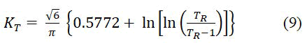
Where, TR is the return period (2, 5, 10, 25, 50 and 100) years.
In the log Pearson type III, it’s a statistical method that can be used for fitting data of frequency distribution to predict the design flood of a stream at a specific location. The merit of this procedure is that the extrapolation is made for the events values with return periods well behind the recorded events of flood. Log Pearson type III is given by equation

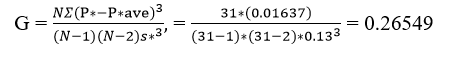
Where, P* ave is the average of P* values, P* is the logarithm of precipitation, S* is the standard deviation of P* values and parameter KT is Pearson frequency factor which depends on return period (TR) and Skewness Coefficient (SC). Values of KT factor can be obtained from Table 2. Skewness coefficient can be calculated by using equation.

Where N is the sample size (number of years of record).
| Frequency factor KT | |||||||
| Â Duration (minutes) | Cs | Return period | |||||
| 2 | 5 | 10 | 25 | 50 | 100 | ||
| 5 | 1.091564 | -0.17865 | 0.746097 | 1.340916 | 2.06406 | 2.581372 | 3.081517 |
| 10 | 0.366734 | -0.06068 | 0.818661 | 1.314339 | 1.869688 | 2.244367 | 2.591381 |
| 15 | 0.251671 | -0.04178 | 0.8269 | 1.305134 | 1.834018 | 2.185869 | 2.509203 |
| 20 | 0.305351 | -0.05086 | 0.823572 | 1.309428 | 1.850659 | 2.213676 | 2.547799 |
| 30 | 0.272066 | -0.04525 | 0.825676 | 1.306765 | 1.840341 | 2.196474 | 2.523888 |
| 45 | -0.15695 | 0.026112 | 0.848278 | 1.263166 | 1.695498 | 1.968677 | 2.209856 |
| 60 | -0.09628 | 0.016367 | 0.845851 | 1.270447 | 1.717303 | 2.002011 | 2.254756 |
| 90 | 0.051879 | -0.00882 | 0.838887 | 1.287188 | 1.768639 | 2.081496 | 2.36439 |
| 120 | -0.2684 | 0.044629 | 0.852052 | 1.249108 | 1.654691 | 1.907378 | 2.127382 |
| 180 | 1.037152 | -0.16994 | 0.75317 | 1.340372 | 2.051545 | 2.557975 | 3.046149 |
| 240 | 1.115837 | -0.18238 | 0.742941 | 1.340842 | 2.069326 | 2.591493 | 3.096819 |
| 300 | 1.232979 | -0.19995 | 0.727713 | 1.33967 | 2.093926 | 2.639191 | 3.169447 |
| 420 | 1.209953 | -0.19649 | 0.730706 | 1.3399 | 2.08909 | 2.629981 | 3.155171 |
Table 2: Log-Pearson frequency factors for various durations and return periods source.
Then, the rainfall intensity IT (in mm/h) for return period TR is obtained by equation

Where PT is the antilogarithm of PT* that obtained by Equation 10
In Lognormal method it follows the same steps of log Pearson type III (i.e., logarithm values of the statistical variables) but with normal KT that was used in the method of Gumbel.
It follows the same steps of LPT III (i.e., logarithm values of the statistical variables) but with normal KT that was used in the method of Gumbel.
A researcher implemented an Indian Meteorological Department (IMD) which uses an empirical reduction formula (Equation 13) for estimation of various duration like 1 hr, 2 hr, 3 hr, 5 hr, 6 hr and 12 hr rainfall values from annual maximum values again IMD empirical reduction formula was used to estimate the short duration rainfall from daily rainfall data in Sylhet city and found that this formula gives the best estimation of short duration rainfall [7]. In this study this empirical formula is used to estimate short duration rainfall in Doyogena catchment is given by:

Where, Pt is the required rainfall depth in mm at t-minute duration
P24 is the daily rainfall in mm
t is short duration in minute
Result of existing drainage system based on their type
The general characteristics of existing drainage system of the study area are classified on some factors based on their types like their shape, depth and others surface materials. The length of existing drainage system, out of the total constructed length which covers 13.806 km. When seen regarding to their shape, the existing drainage structures are classified into different types. This included rectangular and trapezoidal shapes, are discovered through field observation from which only 27.72 percent of the drainage structures are rectangular shape and whereas 72.28 percent of these drainage structures are trapezoidal shape as shown in Figure 2. Both rectangular and trapezoidal shapes offer benefits and drawbacks. Compared to rectangular drainage structures, trapezoidal drainage structures require more space. Compared to trapezoidal drainage structures, rectangular drainage structures have a lower capacity.

Figure 2: Types of existing drainage system based on their shape.
Based on the depth of existing drainage system
The depth of the existing drainage structure is assessed during a field survey to determine the general characteristics of the drainage system. The present drainage structures have a depth range of 0.36 meters to 1.5 meters. According to Figure 3, approximately 25.83 percent of these structures have a depth of 0.79 meters, 23.89 percent have a depth of 1.09 meters, 19.13 percent have a depth of 0.36 meters and 31.15 percent have a depth of 0.9 meters.
Also the exact dimensions of the side drains are dependent on the expected amount of rainwater and the distance to the next exit point where the water can be diverted away from the road. Rectangular drainage structures must have a depth of at least 0.75 meters, but in the town of Doyogena, certain drainage structures have a depth of fewer than 0.75 meters, failing to meet the requirements of the ERA manual.

Figure 3: Types of existing drainage system based on its depth.
Based on surface material
Knowing the surface material from which a drainage structure was built is essential when calculating the discharge value since different construction materials have varied rainfall run-off coefficients. Therefore, during the investigation, the nature of such construction materials was determined by observation and reports from the town's municipality office. According to their report and what is observed on the ground, 27.72 percent of the drainage structures are made of gravel with mortar at the bottom and masonry at the sides and 72.28 percent are made of concrete, as shown in Figure 4.

Figure 4: Classes of existing drainage system based on construction materials.
Terrain category of the Doyogena town
Using Arc GIS software, the topography type of the town is categorized according to the standard. These divisions are made by the study area's slope variations. The town's DEM data is acquired from the USGS wave site for this categorization and the study area's DEM is then extracted from this DEM data by the study area shape file. This DEM is used to classify the town's slope, using ArcGIS software. According to this classification terrain category of the town lies between plain and steep which is shown in the Figure 5.

Figure 5: Town cross slope.
Drains should have a longitudinal slope between 2% and 5% on flat or lightly undulating terrain. Gradients less than 2% easily cause silting, whereas those greater than 5% quickly cause ditches to erode. To reduce the flow of water on steep slopes, use rubble, riprap or fabric can also pave the slopes to stop severe erosion. A quick storm sewer installation could also be taken into consideration. However, because practically all computed slopes have values greater than 5%, there are drainage structures that are vulnerable to erosion because of steep slopes [8].
Goodness-of fit tests by using Esay Fit software
Kolmogorov-Smirnov, Anderson-Darling as well as chi-squared this are the three goodness of fit test methods. It will give statistics as well as rank as you can see in Table 3 for Kolmogorov-Smirnov our rank is Weibull where as if we select Anderson-Darling statistics method you can select Gumbel max. But if we select chi-squared statistics method you can select Inv. Gaussian method. So here under Anderson-Darling and select Gumbel max so our data only Gumbel. Finally select Gumbel method.
| Gumbel Max | |||||
| Kolmogorov-Smirnov | |||||
| Sample size | 31 | ||||
| Statistic | 0.11777 | ||||
| P-value | 0.73949 | ||||
| Rank | 6 | ||||
| α | 0.2 | 0.1 | 0.05 | 0.02 | 0.01 |
| Critical value | 0.18732 | 0.21412 | 0.23788 | 0.26596 | 0.2853 |
| Reject? | No | No | No | No | No |
| Anderson-Darling | |||||
| Sample size | 31 | ||||
| Statistic | 0.41148 | ||||
| Rank | 1 | ||||
| α | 0.2 | 0.1 | 0.05 | 0.02 | 0.01 |
| Critical value | 1.3749 | 1.9286 | 2.5018 | 3.2892 | 3.9074 |
| Reject? | No | No | No | No | No |
| Chi-Squared | |||||
| Deg. of freedom | 3 | ||||
| Statistic | 0.30202 | ||||
| P-value | 0.95965 | ||||
| Rank | 8 | ||||
| α | 0.2 | 0.1 | 0.05 | 0.02 | 0.01 |
| Critical value | 4.6416 | 6.2514 | 7.8147 | 9.8374 | 11.345 |
| Reject? | No | No | No | No | No |
Table 3: Goodness of fit-details.
The best fit for each distribution is assessed using the chi-square, Anderson–Darling and Kolmogorov-Smirnov fit test for each period using easy fit 5.5. With the help of a quality fit test and LSSMIC, the best appropriate distribution has been determined. The results showed that the best distribution is Gumball method as shown in Table 4.
| Distribution | Statistics | ||||
| Kolmogorov-Smirnov | Anderson-Darling | Chi-square | LSSMIC | Best fit | |
| Gumball | 0.11777 | 0.41148 | 0.30202 | 0.16873 | Best |
| LPT III | 0.43163 | 0.73363 | 0.60893 | 0.77421 | |
| Lognormal | 0.16831 | 0.49546 | 0.54263 | 0.2064 | |
Table 4: Best fit model.
Gumbel distribution
It determines the return period intervals of 2, 5, 10, 25, 50 and 100 years for every duration, it needs many calculations. For every duration with a certain return period Tr (in a year), rainfall frequency Pt (in mm) can be determined. After that, the intensity of rainfall IT (in mm/h) for Tr return period can be achieved. The results obtained in Table 5 revealed that the rainfall intensity reduces as storm duration increases. Furthermore, rainfall of a certain duration has a higher intensity when it has a high return period. Figure 6 shows the IDF curves for the Gumbel method. These curves are plotted on the normal scale for Gumbel methods (for Tr=2, 5, 10, 25, 50 and 100 years).
| T | KT | PT | IT | PT | IT | PT | IT |
| 2 | -0.164 | 0.32 | 0.64 | 29.29 | 29.29 | 4.85 | 0.2 |
| 5 | 0.719 | 0.54 | 1.08 | 74.34 | 74.34 | 34.61 | 1.44 |
| 10 | 1.304 | 0.69 | 1.37 | 104.19 | 104.19 | 9.4 | 0.39 |
| 25 | 2.04 | 0.87 | 1.74 | 141.74 | 141.74 | 11.68 | 0.49 |
| 50 | 2.592 | 1.01 | 2.02 | 169.9 | 169.9 | 13.4 | 0.56 |
| 100 | 3.137 | 1.14 | 2.29 | 197.71 | 197.71 | 15.08 | 0.63 |
Table 5: Computed Intensity (IT) in (mm/h) (Gumbel method)

Figure 6: IDF curves for the study area (Gumbel method).
LPT III distribution
The LPT III distribution model can be applied to determine the precipitation intensities for different return periods and precipitation durations from historical IDF curves. The LPT III distribution includes the logarithms of the computed values. The precipitation frequency is calculated by the LPT III procedure using equation (30), as shown in Table 6 shows the computed values of KT for Tr=2, 5, 10, 25, 50 and 100 years that lead to calculate the frequency rainfall depth Table 5. To estimate floods in rural/urban basins, the resulted curves of IDF can be used. Using the resulted curves of IDF is recommended for the safe, efficient and rigorous design of flood protection projects and hydraulic structures. Thus, the obtained IDF curves can be used, as displayed in (Figures 7 and 8 and Tables 7,8).
| Year | P (mm) | P*=Log p | P*ave | (P*-P*ave)2 | (P*-P*ave)3 |
| 1990 | 42 | 1.62 | 1.68 | 0.0028 | -0.00015 |
| 1991 | 44.5 | 1.65 | 1.68 | 0.0008 | -0.00002 |
| 1992 | 57 | 1.76 | 1.68 | 0.0064 | 0.00051 |
| 1993 | 35 | 1.54 | 1.68 | 0.0174 | -0.00229 |
| 1994 | 32.7 | 1.51 | 1.68 | 0.026 | 0.00419 |
| 1995 | 61.3 | 1.79 | 1.68 | 0.0125 | -0.00139 |
| 1996 | 39.5 | 1.6 | 1.68 | 0.0063 | -0.0005 |
| 1997 | 61 | 1.79 | 1.68 | 0.012 | 0.00131 |
| 1998 | 53 | 1.72 | 1.68 | 0.0024 | 0.00011 |
| 1999 | 37.5 | 1.57 | 1.68 | 0.0104 | -0.00105 |
| 2000 | 50 | 1.7 | 1.68 | 0.0005 | 0.00001 |
| 2001 | 44.5 | 1.65 | 1.68 | 0.0008 | -0.00002 |
| 2002 | 30 | 1.48 | 1.68 | 0.0395 | -0.00784 |
| 2003 | 39 | 1.59 | 1.68 | 0.0072 | -0.00061 |
| 2004 | 30.5 | 1.48 | 1.68 | 0.0367 | -0.00702 |
| 2005 | 30.5 | 1.48 | 1.68 | 0.0367 | -0.00702 |
| 2006 | 50 | 1.7 | 1.68 | 0.0005 | 0.00001 |
| 2007 | 90.5 | 1.96 | 1.68 | 0.0789 | 0.02215 |
| 2008 | 51 | 1.71 | 1.68 | 0.001 | 0.00003 |
| 2009 | 60 | 1.78 | 1.68 | 0.0105 | 0.00107 |
| 2010 | 44 | 1.64 | 1.68 | 0.001 | -0.00003 |
| 2011 | 94 | 1.97 | 1.68 | 0.0884 | 0.02629 |
| 2012 | 52 | 1.72 | 1.68 | 0.0016 | 0.00006 |
| 2013 | 50 | 1.7 | 1.68 | 0.0005 | 0.00001 |
| 2014 | 56 | 1.75 | 1.68 | 0.0052 | 0.00038 |
| 2015 | 30 | 1.48 | 1.68 | 0.0395 | -0.00784 |
| 2016 | 58.5 | 1.77 | 1.68 | 0.0083 | 0.00076 |
| 2017 | 55 | 1.74 | 1.68 | 0.0042 | 0.00027 |
| 2018 | 60 | 1.78 | 1.68 | 0.0105 | 0.00107 |
| 2019 | 38 | 1.58 | 1.68 | 0.0092 | -0.00089 |
| 2020 | 56 | 1.75 | 1.68 | 0.0052 | 0.00038 |
| Average=49.45 | Average=1.68 | Σ=0.4827 | Σ=0.01637 | ||
| Standardization=0.13 | |||||
Table 6: Statistical variables calculated using LPT III.
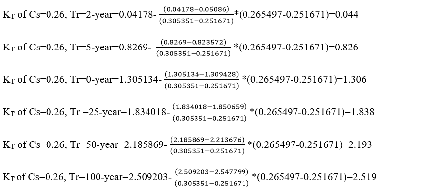
To find KT, we need to know return period (Tr ) and Skewness Coefficient (Cs).
Interpolation
| Frequency factor KT | ||||||
| Skewness coefficient (Cs) 0.26 | Return period | |||||
| 2 | 5 | 10 | 25 | 50 | 100 | |
| 0.044 | 0.826 | 1.306 | 1.838 | 2.193 | 2.519 | |
Table 7: Calculated Pearson frequency factor (KT) depending on skewness coefficient and return period.
| T | KT | PT* | PT | IT | PT* | PT | IT | PT* | PT | IT |
| 2 | 0.044 | 0.46 | 2.88 | 5.76 | 0.58 | 3.8 | 3.8 | 1.69 | 48.98 | 2.04 |
| 5 | 0.826 | 0.48 | 3.02 | 6.04 | 0.61 | 4.07 | 4.07 | 1.79 | 16.66 | 2.57 |
| 10 | 1.306 | 0.5 | 3.16 | 6.32 | 0.63 | 4.26 | 4.26 | 1.85 | 70.79 | 2.95 |
| 25 | 1.838 | 0.52 | 3.31 | 6.62 | 0.65 | 4.47 | 4.47 | 1.92 | 83.18 | 3.47 |
| 50 | 2.193 | 0.53 | 3.39 | 6.78 | 0.67 | 4.68 | 4.68 | 1.97 | 93.32 | 3.89 |
| 100 | 2.519 | 0.54 | 3.47 | 6.94 | 0.68 | 4.79 | 4.79 | 2.01 | 102.33 | 4.26 |
Table 8: Computed intensity (IT) in (mm/h) (LPT III method).

Figure 7: Rainfall intensity IDF curves (LPT method).
Log normal distribution
Different type of calculated intensity shows in Table 9.
| T | KT | PT* | PT | IT | PT* | PT | IT | PT* | PT | IT |
| 2 | -0.164 | 0.46 | 2.88 | 5.76 | 0.57 | 3.71 | 3.71 | 1.66 | 45.71 | 1.9 |
| 5 | 0.719 | 0.48 | 3.02 | 6.04 | 0.61 | 4.07 | 4.07 | 1.77 | 58.88 | 2.45 |
| 10 | 1.304 | 0.5 | 3.16 | 6.32 | 0.63 | 4.26 | 4.26 | 1.85 | 70.79 | 2.95 |
| 25 | 2.04 | 0.52 | 3.31 | 6.62 | 0.66 | 4.57 | 4.57 | 1.95 | 89.12 | 3.71 |
| 50 | 2.592 | 0.54 | 3.47 | 6.94 | 0.68 | 4.79 | 4.79 | 2.02 | 104.71 | 4.36 |
| 100 | 3.137 | 0.55 | 3.55 | 7.1 | 0.71 | 5.13 | 5.13 | 2.09 | 123.03 | 5.13 |
Table 9: Calculated intensity (IT) in (mm/h) (lognormal method).

Figure 8: Rainfall intensity IDF curves (lognormal method).
Deriving intensity duration frequency relationship of rain fall at town
Intensity-Duration-Frequency (IDF) curves describe the relationship between rainfall intensity, rainfall duration and return period (or its inverse, probability of exceedance). IDF curves are commonly used in the design of hydrologic, hydraulic and water resource systems. It also used in conjunction with run off estimation formula: The rational method, to predict the peak run off amounts from a watershed. The information from the curves is then used in hydraulic design to size urban drainage work. The curves obtained by using Gumball distribution methods for station provide for a given return period and duration the rain intensities at any point in the basin.
Figure 9 show the IDF curve for 24-hour maximum rain fall to obtain crucial information for design, capacity estimation, performance evaluation, risk analysis and climate change considerations. It also ensures that drainage infrastructure is appropriately designed, maintained and able to handle the expected run off during rain fall events [9].

Figure 9: Rain fall IDF curve.
Based on these to estimate the maximum rainfall intensity for different duration and return period the following empirical equation is used i=x × (td)-y
Where,
i=Rainfall intensity in mm/hr
td=Rainfall duration in minutes
x and y are the parameters to fit the IDF curve
Least square method is applied to get parameters x and y for various return periods and the outcomes are shown in the below Table 10 of rainfall intensity-duration-frequency empirical equation for corresponding return period and their correlation coefficients for meteorological stations.
| Return period | Rain falls (XT)=Ay+B | A | B |
|
Rain falls intensity (i)=XT*(td)-y |
Correlation coefficient |
| 2 | 47 | 12 | 43 | 0.4 | 47*(td)-0.4 | 0.97 |
| 5 | 61 | 1.5 | 61*(td)-1.5 | 0.97 | ||
| 10 | 70 | 2.3 | 70*(td)-2.3 | 0.97 | ||
| 20 | 78 | 3 | 78*(td)-3 | 0.97 | ||
| 30 | 83 | 3.4 | 83*(td)-3.4 | 0.97 | ||
| 50 | 89 | 3.9 | 89*(td)-3.9 | 0.97 | ||
| 100 | 98 | 4.6 | 98*(td)-4.6 | 0.97 |
Table10: Least square method.
Estimation of short duration rainfall
All the computation in the Table 11 below has been done by use of Microsoft excel program function to estimate the short duration rainfall from expected maximum rain fall data.
| Tr year | Highest rain falls (mm) | 10 min | 20 min | 30 min | 60 min | 120 min | 180 min | 360 min | 720 min | 1440 min |
| 2 | 47 | 9 | 11 | 13 | 16 | 21 | 24 | 30 | 37 | 47 |
| 5 | 61 | 12 | 15 | 17 | 21 | 27 | 31 | 38 | 48 | 61 |
| 10 | 70 | 13 | 17 | 19 | 24 | 31 | 35 | 44 | 56 | 70 |
| 20 | 78 | 15 | 19 | 21 | 27 | 34 | 39 | 49 | 62 | 78 |
| 30 | 83 | 16 | 20 | 23 | 29 | 36 | 42 | 52 | 66 | 83 |
| 50 | 89 | 17 | 21 | 24 | 31 | 39 | 45 | 56 | 71 | 89 |
| 100 | 98 | 19 | 24 | 27 | 34 | 43 | 49 | 62 | 78 | 98 |
| Mean | 14 | 18 | 21 | 26 | 33 | 38 | 47 | 60 | 75 | |
| Standard deviation | 3.3 | 4.2 | 4.8 | 6 | 7.6 | 8.7 | 11 | 14 | 17 |
Table 11: Short-duration rain falls data derivation from max daily rainfall using IMD 1/3rd rule.
Hydraulic performance of existing drainage system
Existed drainage channels and their hydraulic carrying capacity shows in Table 12.
| Channel Id | 1 | 2 | 3 | 4 | 5 | 6 | 7 | 8 |
| Drainage type | Trapezoidal | Rectangular | Rectangular | Rectangular | Rectangular | Rectangular | Trapezoidal | Rectangular |
| Cross-section data | W=0.4 | W=1.23 | W=1.65 | W=0.8 | W=0.85 | W=0.68 | W=0.4 | W=1.5 |
| Y=0.3 | Y=1.17 | Y=1.5 | Y=0.75 | Y=0.73 | Y=0.86 | Y=0.3 | Y= 1.2 | |
| Area (m2) | 0.3 | 1.44 | 2.48 | 0.6 | 0.62 | 0.59 | 0.3 | 1.8 |
| Perimeter (m) | 1.74 | 3.57 | 4.65 | 2.3 | 2.31 | 2.4 | 1.74 | 3.9 |
| Hydraulic radius (m) | 0.17 | 0.4 | 0.53 | 0.26 | 0.27 | 0.24 | 0.17 | 0.46 |
| Slope | 0.04 | 0.08 | 0.037 | 0.103 | 0.08 | 0.082 | 0.08 | 0.034 |
| Roughness coefficient | 0.023 | 0.023 | 0.023 | 0.023 | 0.023 | 0.023 | 0.023 | 0.023 |
| Side slope | 1v:2h | 1v:1h | 1v:1h | 1v:1h | 1v:1h | 1v:1h | 1v:2h | 1v:1h |
| Velocity (m/s) | 2.59 | 2.12 | 5.49 | 5.7 | 5.25 | 4.86 | 3.85 | 4.79 |
| Discharge (m3/s) | 1.78 | 3.05 | 13.59 | 3.42 | 3.26 | 2.84 | 1.16 | 8.62 |
Table 12: Existed drainage channels and their hydraulic carrying capacity.
The working spaces of the various drainage structure types in the catchments of the research region are shown in Table 13 above which is created using (tap meters) and measurements of the roughness coefficients, side slopes and bed slopes. Finally, manning formulae have been used to estimate the carrying capacity of the drainage structures.
| Col (1) | Col (2) | Col (3) | Col (4) | Col (5) | Col (6) | ||
| Catch Id | Area (ha) | Run-off coefficient | Time of concentration (min) | Intensity (mm/ha) | Proposed peck discharge Q=0.00278 CIA | ||
| 5-yrs | 10-yrs | 5-yrs | 10-yrs | ||||
| Sca-1 | 4.11 | 0.8 | 0.63 | 122 | 203 | 1.11 | 1.85 |
| Sca-2 | 2.95 | 0.8 | 0.67 | 111 | 176 | 0.73 | 1.15 |
| Sca-3 | 3.94 | 0.8 | 0.35 | 295 | 783 | 2.58 | 6.86 |
| Sca-4 | 4.28 | 0.5 | 0.36 | 282 | 734 | 1.68 | 4.36 |
| Sca-5 | 4.08 | 0.5 | 0.38 | 260 | 648 | 1.48 | 3.68 |
| Sca-6 | 4.15 | 0.5 | 0.41 | 232 | 544 | 1.34 | 3.14 |
| Sca-7 | 5.83 | 0.8 | 0.6 | 131 | 227 | 1.7 | 2.94 |
| Sca-8 | 4.66 | 0.5 | 0.47 | 189 | 397 | 1.23 | 2.57 |
Table 13: Computation of the maximum discharge suggested by the study area's using rational formula.
The proposed maximum discharge computations are shown in Table 13, it is existed drainage system above where column one shows the Id of sub-catchment area in the study area, column two shows the sub catchment area in hectare, column three shows the run off coefficient, column four shows the time of concentration, column five shows the rain fall intensity for different return period, and column six shows the proposed peak discharge for the different return period (Table 14).
| Col (1) | Col (2) | Col (3) | Col (4) | Col (5) | ||
| Channel Id | Total discharge | Existed channel capacity | Proposed peck discharge | Difference discharge | ||
| Q, design 5-yr | Q, check 10-yr | Q, design 5-yr | Q, check 10-yr | |||
| Sch-1 | Q1 | 0.78 | 1.11 | 1.85 | 0.33 | 1.07 |
| Sch-2 | Q1+Q3+Q2 | 3.05 | 4.42 | 9.86 | 1.37 | 6.81 |
| Sch-3 | Q3 | 13.59 | 2.58 | 6.86 | -11.01 | -6.73 |
| Sch-4 | Q4 | 3.42 | 1.68 | 4.36 | -1.74 | 0.94 |
| Sch-5 | Q5 | 3.26 | 1.48 | 3.68 | -1.78 | 0.42 |
| Sch-6 | Q6 | 2.84 | 1.34 | 3.14 | -1.5 | 0.3 |
| Sch-7 | Q7 | 1.16 | 1.7 | 2.94 | 0.54 | 1.78 |
| Sch-8 | Q6+Q7+Q8 | 8.62 | 4.27 | 8.65 | -4.35 | 0.03 |
Table 14: Comparison of proposed peak design discharge and their existing drainage structure capacity.
The computed proposed peak discharge shown in Table 13 and the carrying capacity of existing drainage structures shown in Table 12 indicate that most of existing drainage structures require rehabilitation.
The contrast between the existing drainage infrastructure and the suggested maximum design discharge on the catchment is made obvious in Table 14, which is previously mentioned (Table 15).
| Catchment ID | % of flood over flow on the road | |
| Q (m3/s) 5-year design | Q (m3/s) 10-year check | |
| S.cm-1 | 29.73% | 57.84% |
| S.cm-2 | 30.99% | 69.07% |
| S.cm-3 | 0% | 0% |
| S.cm-4 | 0% | 21.56% |
| S.cm-5 | 0% | 11.41% |
| S.cm-6 | 0% | 9.55% |
| S.cm-7 | 31.76% | 60.54% |
| S.cm-8 | 0% | 0.35% |
Table 15: Percentage of the flood which overtopped and flows on the road.
The overtopped discharge directly affects the performance of the road and creates an environmental problem [10].
Existed culverts analysis using HY8 software
Different type of parameters existed culverts analysis using HY8 software (Table 16).
| Parameter | Value | Units |
| Design discharge | Q10 yr | m3/s |
| Roadway crest elevation | 2 | m |
| Roadway top width | 20 | m |
| Culvert length | 25 | m |
| Culvert shape | Box (circular) | |
| Culvert material | Concrete (manning’ss n=0.012) | |
| Culvert inlet elevation | 2592 | |
| Culvert outlet elevation | 2591.92 | m |
| Number of barrels | 1 | no’s |
| Culvert station | 257+294 | m |
| Initial culvert sizing | 900 | mm |
Table 16: Design parameters.
Doyogena town is one of newly fast developing towns found in SNNPR state in Ethiopia; there are many lacks of quality infrastructures mostly regarding water flow and drainage system constructions. It needs high concern of government, community and NGOS to support with budget, high follow up and supervision to sustain existing and to construct new with standard quality. These has in forced the researcher to give high concern to solve the continuing problem of the town by conducting a legal study work as one of the inhabitant persons of this town especially on drainage problems. In order to this the study gave high concern on collecting data by using both qualitative and quantitative methods that enabled to get enough data source from those institutions, individuals, previews paper works of universities and soon.
This study is focused on that the general characteristics of existed drainage structure at Doyogena town are identified during field observation that general characteristics are based on types of existing drainage structure from which 72.28% is trapezoidal while 27.72% rectangular, based on its depth 25.83% of drainage structures depth is 0.79 m, 23.89% drainage structure depth is 1.09 m, 19.13% is 0.36 m and 31.15% is 0.9 m. Based on its construction material 72% of drainage structures is concrete, 28% of drainage structure is masonry. Moreover; there are different functional classes of roads in the town which have different surfacing material like: Earthen roads, compacted earthen, gravel, cobblestone and asphalt roads. Also, there are sidewalks of 38.10 km gravel, 3 km cobble stone and 80% is compacted earthen surface materials. Since the terrain category of the area is plain and steep water flow on the surface of unpaved roads and sidewalk with high speed which is resulting erosion on the surface of those roads and sidewalk are damaging them.
Some drainage structure releases the water to farmlands of the farmers; some of them release water to residential while others release it to some other structures like roads. This drainage structures which releases water to other facilities are damaging the structures and the surrounding farmers were block those structures which release water to their farms to protect their farm from damage. Secondly; in this study the terrain category of the town was classified by using ArcGIS software, based on standard and the slope of the terrain category of this town ranges between 0% to 65%, which is plan and steep terrain category. The terrain category affects the longitudinal slope of the drainage structure. At this terrain category the longitudinal slope of the drainage structure should be less than 5 percent. Unless this criterion does not achieve erosion can be resulted. This defect is highly observed in the Doyogena town. During field observation erosion are observed with in the drainage structure.
In general, to identify the causes this erosion the slopes of each drainage segment are calculated and the slope ranges between 0.8 percent and 10.3 percent but as stated above the longitudinal slope of the drainage structure must be less than 5 percent, since the terrain category of the town is flat and steep. Due to this the longitudinal slope of the existing drainage structure, can be a factor of erosion in this town. Siltation is not only due to flat slope but also, composition of west in the drainage structure and blocked drainage structure, plant growing in the drainage structure is also another factor. During the study, the capacity of existing drainage structure is also checked and it is identified that the capacity of some existing drainage structure is less than the discharge value or required capacity while others are greater than the required capacity. Due to this both siltation and inadequate existing drainage capacity are identified as factor that causing street flood in the Doyogena town.
Citation: Yosef NE, Ayele EG, Garo OO (2025) Assessment of Hydraulic Performance of Drainage System: In Doyogena Town, Kembata Zone-Ethiopia. J Res Dev. 13:292.
Received: 30-May-2024, Manuscript No. JRD-24-31765; Editor assigned: 04-Jun-2024, Pre QC No. JRD-24-31765 (PQ); Reviewed: 18-Jun-2024, QC No. JRD-24-31765; Revised: 03-Apr-2025, Manuscript No. JRD-24-31765 (R); Published: 10-Apr-2025 , DOI: 10.35248/2311-3278.25.13.292
Copyright: © 2025 Yosef NE, et al. This is an open-access article distributed under the terms of the Creative Commons Attribution License, which permits unrestricted use, distribution, and reproduction in any medium, provided the original author and source are credited.
