Journal of Geology & Geophysics
Open Access

Assessing Spatial Heterogeneity of Soil Properties under Sugarcane Cropping System using Geostatistical Models and GIS Techniques

Author info »

Introduction

Understanding the spatial variability of the soil properties entails soil fertility evaluation and refining agricultural practices. Spatial heterogeneity of soil is inherent in nature due to geologic and pedologic soil forming factors yet different land uses and management practices had a considerable impact on soil properties degradation. Soil nutrient deficiency is one of the prime restraints on crop production because of crop intensification, and enhanced application of macronutrients with less or nil micronutrients. The widespread micronutrient deficiency in different parts of a country may continuously be assessed and maps prepared from geostatistics. These deficiency maps help policymakers and fertilizers industries for acconting the supply and demand of a particular area, and it also useful in micronutrient management with the right nutrient, amount, form, and place of application which enhances the crop production and soil health [1].

Geostatistics has been manifested as a useful tool for assessing spatial variability of soil properties and has crucial importance in the near future for diagnosing nutrient related limitations and their management. Assessment of spatial interpolation which involves ordinary or co-kriging techniques paves way for forecasting the variable at unknown points with known sampling data. It is developed to create a mathematical model of spatial correlation structures with variogram construction both isotropically and anisotropically. The variogram and kriging are the most commonly used geostatistics and interpolation techniques which disclose the best-unbiased result and good fit determined by least square sense. Spatial variance data are characterized and modeled with the aid of semi-variograms and cross-semi variograms that assess the data points related to separation distances and through kriging predicted and observed values between samples of modeled variance were estimated. With these techniques, high resolution soil maps which are useful for land use planning and nutrient management for crops can be generated [2].

Stepwise Multiple Linear Regression (SMLR) is one of the popular statistical algorithms for weighing spatial soil information prediction. To determine the interrelationship between available micronutrients and soil characteristics the simple correlation and step-wise multiple regression coefficients were also worked out between certain interrelated pairs of parameters to observe their degree of dependence. Principal Component Analysis (PCA) is a multivariate statistic that provides effective components from other auxiliary variables by reducing multidimensional data into small number orthogonal linear combinations [3].

Materials and Methods

Study area

Sivagangai district is located in the South of Tamil Nadu and it is bounded on the North and Northeast by Pudukkottai district, on the Southeast and South by Ramanathapuram district, on the Southwest by Virudhunagar district, and on the west by Madurai district, and on the Northwest by Tiruchirappalli district. The district has 9 taluks and 12 blocks with a total geographical area of 4189 sq.km between 9°43' and 10°2' North latitude and between 77°47' and 78°49' East longitude with the altitude of 108 M above sea level. The district enjoys a tropical climate. The period from April to June is generally hot and dry. The district’s highest day temperature in summer is between 30°C to 36°C. Average temperatures from January to May ranges from 26°C-32°C. The district receives mean annual rainfall of 904.7 mm from North East monsoon. Paddy is the predominant crop of the district and other crops like millets, cereals, pulses, sugarcane and groundnut were also been cultivated.

The detailed soil survey was mainly focused in Thirupuvanam block which is positioned at the southern side of Madurai district. The geographical area of this block is about 1800 ha and the experimental site taxonomically grouped as Typic Ustropept [4].

Soil sampling and laboratory analysis

In the study area, soil sampling sites were randomly selected in major sugarcane growing soils of the Thirupuvanam block. A total of 100 soil samples were collected at a depth of 0 cm-30 cm. A geo-coordinate of the sampling sites was noted with the aid of a handy GPS device. Soil samples are labeled and stored in an airtight polyethylene bag. The soil samples were dried under shade dry conditions and further crushing and sieving processes were performed. By following the standard procedures, the soil samples were analysed for various chemical properties viz., pH (Potentiometry in a soil water suspension of 1:2 ratio Jackson), Electrical conductivity (Conductometry in a soil water suspension of 1:2 ratio), soil organic carbon (Walkley and black method), free CaCO₃ (rapid titration method), and DTPA Zn, Fe, Mn, (DTPA extract-atomic Absorption spectrophotometer) and hot-soluble B (Hot water-soluble method).

Statistical analysis

The datasets were analysed using statistics, geostatistics, and multivariate analysis. Exploration of data was performed using descriptive statistics that help to examine the central tendency and variability. The parameters of descriptive statistics such as mean, median decide the central tendency of the datasets while the minimum, maximum, Standard Deviation (SD), Coefficient of Variance (CV), kurtosis, and skewness decide the variability (spread) of the datasets. Log transformation was performed if the data sets were not normally distributed. The coefficient of variance was used to compute the degree of variability in soil properties. It is categorized into low (<12%), medium (12%-60%), and high (>60%).

Descriptive statistics, multivariate analysis viz., correlation, stepwise multiple linear regression and principal component analysis were carried out using IBM SPSS statistical version 22 and Microsoft excel 2007. Semi-variance analysis was carried out to quantitively determine the spatial dependence levels of the variable using Arc GIS 10.8 software. A semi-variogram was calculated for each property as follows [5].

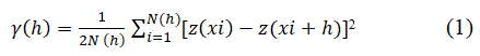
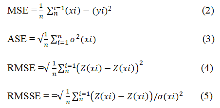
Different semi-variogram models were used for each soil property such as the circular model, gaussian model, exponential model, and spherical model. The model fitting was recognized by adopting cross-validation techniques which evaluate the performance of the selected interpolated methods. It also computes the prediction error of the map viz., Mean Square Error (MSE), Average Standard Error (ASE), Root-Mean- Square Error (RMSE) and the Standardized Root Mean Square Error (RMSSE). They are defined as follows:

The least Residual Sum of Squares (RSS) was taken into account to assess the most reliable interpolation method. In some cases, where these parameters were equal, the mean square error value closest to zero was used. The Degree of Spatial Dependence (DSD) of the variables were concerned based on the ratio of nugget effect to sill. The nugget effect (C0) reflects the spatial variability of the random field and the sill (C0+C) denotes the total variation, whereas the Range (R) indicates the separation distance, after which the measured data are not spatially dependent, the Degree of Spatial Dependence (DSD) was classified into DSD ≤ 25% strong; 25<DSD ≤ 75% moderate, and DSD>75% weak. The best-fitted model was further preceded to interpolation using the ordinary kriging method and the thematic maps on each soil property were generated [6].

Results and Discussion

Descriptive statistics

The summary statistics of the surface soil attributes was revealed in Table 1. From these results, it is evident that the soil pH ranges from 6.5-8.5 which falls under the category of slightly acidic to slightly alkaline and non-saline. The concentration of soil organic carbon varied from 3.10 (low)-7.80 g kg^-1 (medium). The free calcium carbonate content of surface soils was in the range of 0.30 (non-calcareous) -5.90% (slightly calcareous).

Availability of micronutrients B, Fe, Cu, Zn, and Mn ranged from deficiency level to sufficiency level. The skewness and kurtosis of the variable emphasize the asymmetric distribution of the data sets. The variable with positive skewness represents the wider limits on the variogram and the least variance reliability.

The magnitude of skewness for pH and EC contents were negatively skewed or left skewed which depicts that most of the values are concentrated on the right tail of the distribution graph and asymmetry is present on the left side. Other attributes were positively skewed where the asymmetry fall on the right side. On the other hand, the Zn and B showed a positive kurtosis, whereas the others had a negative one. Based on the Standard Deviation (SD) value, the maximum and minimum dispersion in datasets were noticed in Fe and EC respectively. The Coefficient of Variation (CV) value ranges from low (7.32%) to moderate (49.83%) based on the classification proposed by Warrick and Nielson. The lowest and highest values were obtained for pH and B respectively. The variation in the soil properties is due to heterogeneity in nutrient levels in surface soil and topographical variation and different management practices. Similar results have been reported by Ranjbar and Jalali (Table 1) [7].

Table 1: Descriptive statistics for the soil attributes.

Relationship between soil properties and nutrient availability

Simple correlations and stepwise multiple linear regression were worked out to establish the relationship between available micronutrients and other soil properties viz., pH, EC, OC, and CaCO₃ of the soil samples. The correlation coefficient and R2 are presented in Tables 2 and 3. Soil pH had a significant and positive correlation with OC (r=0.044), free CaCO₃ (r=0.069) and whereas it had a negative correlation with EC (r=-0.350) and available B (r=-0.090), available Fe (r=-0.326), Cu (r=-0.477), Zn (r=-0.674), and Mn (r=-0.771). Followed by it, EC was negatively correlated with available Fe (r=-0.046), Cu (r=-0.302), Zn (r=-0.371), Mn (r=-0.338), and positively correlated with organic carbon (r=0.093), free CaCO₃ (r=0.029) and available boron (r=0.007). Regarding soil organic carbon, it had a significant and positive correlation with available Fe (r=0.062), Zn (r=0.123), Cu (r=0.062), B (r=0.009), and Mn (r=0.081). Finally, considering the free calcium carbonate, it showed a highly significant and negative correlation with Fe (r=-0.086), Cu (r=-0.134), Mn (r=-0.015), and available B (r=-0.073). The results showed that available B had 96% of variation was explained by combination of pH, EC, organic carbon, free CaCO₃ followed by Mn (93%), Zn (92%), Cu (90%) and Fe (85%) (Table 2) [8].

Table 2: Pearson correlation matrix between soil properties and nutrient availability.

Table 3: Stepwise multiple regression between micronutrients and soil pH, EC, OC, and CaCO₃.

Zn, Cu, Fe, Mn, and B are negatively correlated with soil pH. In the alkaline range >7.85, the hydroxides of zinc are formed. Negative correlations between Cu and pH are probably due to the precipitation of Cu as hydroxides at high pH would have either the part of the lattice or occluded with the hydroxides of Fe, Al, and Mn. The reduction in availability of Fe is due to the conversion of Fe²⁺ ions to Fe³⁺ ions and the formation of Fe (OH)₂ under a high pH range. Divalent (Mn²⁺) form of Mn get converts into insoluble tri or polyvalent ion (Mn³⁺-, Mn⁷⁺). A negative correlation was observed with increased pH, as the CaCO₃ content increased the adsorption of B increased, and the availability of B in soils reduced. Positive correlation with organic carbon and micronutrients and it is reported that organic matter decomposition provides chelating agents to help in the reduction of soil pH at the soil locality which renders the solubility of micronutrients and their availability get improved. Soil micronutrient dynamics are also governed by organic matter build which influences the sorption mechanism of the micronutrients between soil colloids and solution. Since the organic matter has a highly active functional group, high specific surface area, action exchange capacity and it led to soluble complexes formation. Micronutrients had a negative correlation with calcium carbonate which acts as a strong adsorbent. High calcium carbonate content may lead to precipitation or fixation of nutrients by the adsorption process [9].

Principal component analysis

PCA was performed on variables that decrease the dimensionality of the data and recognize the linear reconsolidation of the properties that conclude the primary drivers of data variability. From the results (Table 4), it was obvious that four principal components (PC1, PC2, PC3, and PC4) pertain to eigenvalues>1 and together elucidated 71.29% of the pattern variance. In PC1, the two highest positive loadings were Mn and Zn followed by the two strongest negative loadings soil pH and EC which explain 33.83% of the structure. In PC2, the positive association was ascribed by B and Fe with 13.78% of the total variance while the organic carbon explained 12.50% of the variation with a positive relationship in PC3. PC4 has a positive impact on free CaCO₃ described 11.16% of the structure. In this connection, the positive loadings decode the contribution of variables that increase with increased dimensional loading and decrease dimensional loading, which depicts negative loading. Similar results were reported by Ali and Ibrahim, Jena et al., Kumar, Lal and Lloyd [10].

Table 4: Results of principal component analysis for soil attributes.

Discussion

Geostatistical analysis

The semi variogram analysis and cross-validation results for the soil properties are presented in Table 5. The best fit model for each property was exponential for pH, EC, Free CaCO₃ and B, Circular model for OC and Zn, spherical for Fe and Mn, and the Gaussian model fitted well for Cu. Each semi-variogram model describes the variation of the soil property. Comparably, the same results were reported for Ph, EC, and Cu. Logarithmic transformation was performed to stabilize the not normally distributed data sets of pH. The nugget, sill, and range decide the semi-variogram construction. The nugget effect determines the continuity at close distances and the highest value registered for Fe (2.990) and OC (1.005) relative to other soil properties. Apparently, the highest nugget value might be due to high soil heterogeneity resulting in the large spatial variability of the nutrients. In the line with the present findings, the soil properties. The lowest nugget value (0.000) was recorded for free CaCO₃ and B. The value of partial sill and sill vary from 0.001-2.217 and 0.003-0.007 respectively. The range value noted for the soil property varies from 0.031 m-0.256 m. From this, it is well known that the higher the range values the more soil uniformity within its own scale. These results conformity with the findings [11].

The nugget/sill ratio describes the spatial dependency which is scaled as: <25% DSD strong; >25-<75% DSD moderate and >75% weak spatial autocorrelation. Free CaCO₃ and B have strong spatial autocorrelation which is associated with changing the intrinsic factors such as parent materials, texture, topography, and mineralogy; extrinsic altering factors such as soil fertilizers and cultivation practices are habitually connected with a weak spatial dependence. The values of micronutrients like Fe, Cu, Zn, and Mn show weak spatial variability. Both intrinsic and extrinsic factors are responsible for moderate spatial dependence while the results of the present study showed that the soil properties pH, EC, and OC noted moderate spatial dependence. These results were in agreement with the findings [12].

The cross-validation approach provides accurate predictions of unknown values of the study area which is used to evaluate semi-variogram models for soil properties. The RMSSE (Root Mean Square Standardized Error) analyzed for all the properties was close to one, indicating a good prediction. The ASE and RMSE values are almost nearer with fewer differences in deciding a good fit agreement for all the properties. By executing these best-fit models and the corresponding semi-variogram parameters, the spatial variability maps were rendered for each soil property (Figures 1-9 and Table 5) [13].

Table 5: Semi-variogram parameters of soil property.

Figure 1: Semi-variograms of soil properties with the lines indicating a best fit model of pH.

Figure 2: Semi-variograms of soil properties with the lines indicating a best fit model of EC.

Figure 3: Semi-variograms of soil properties with the lines indicating a best fit model of organic carbon.

Figure 4: Semi-variograms of soil properties with the lines indicating a best fit model free CaCO₃.

Figure 5: Semi-variograms of soil properties with the lines indicating a best fit model of available Fe.

Figure 6: Semi-variograms of soil properties with the lines indicating a best fit model of available Cu.

Figure 7: Semi-variograms of soil properties with the lines indicating a best fit model of available Zn.

Figure 8: Semi-variograms of soil properties with the lines indicating a best fit model of available Mn.

Figure 9: Semi-variograms of soil properties with the lines indicating a best fit model of available B.

Spatial variability of soil properties

From the Figure 2, the pH of the study area ranges from ≥ 6.5-7.0 (19.3% of the area), 7.1-8.0 (48.2% of area), and 8.1-8.5 (31% of area) which is categorized into neutral to slightly alkaline. Electrical conductivity ranges from 0.32-0.40 (23% of area), 0.27-0.32 (34% of area), and 0.18-0.27 (43%) which simplifies the non-saline soil. This may be due to management practices and inherent soil properties. Soil Organic Carbon (SOC) plays a pivotal role in improving soil properties. SOC status ranges from 3.1-4.6 (39.5% of area), 4.7-5.9 (30% of area), and 6.0-7.8 (28.5% of area) g kg^-1 of SOC. All soils were low to medium in status which may be due to the hyperthermic temperature regime that causes an exponential rate of decomposition which leads to extremely high oxidizing conditions and another reason might be the reduced application of organic matter [14]. As per FAO classification, the status of free calcium carbonate was categorized into non-calcareous (<5%), slightly calcareous (5%-15%), and highly calcareous (>15%). From this, it is well known that the study area was noncalcareous (0.3%-4.9%) in 88.7% of the area and medium (≥ 4.9%-5.9%) in 10.8% of the area. Similar findings also reported in Madurai district with moderate levels of CaCO₃ i.e., 5%-10%. The spatial distribution of micronutrients was categorized as deficient, moderate, and sufficient. The kriged map of Fe exhibited values ranging from 2.20 mg kg^-1-4.0 mg kg^-1(55% of area), 4.1 mg kg^-1-6.0 mg kg^-1 (22.5% of the area), and 6.1 mg kg-1-8.6 mg kg^-1 (20.2% of area). The critical limit of Fe is 3.60 mg kg^-1 below which it is considered deficient. The highest value of Fe (>8.0) could be due to the acidic parent materials. The Cu status was deficient in 52.2% of the area, moderate in 40.5% of the area, and sufficient in 7% of the area. The available Zn ranges from 0.75 mg kg-1-2.50 mg kg-1 was observed and the majority (50.2%) of the area falls under deficient status. Some parts of the soils were slightly alkaline and hold an appreciable amount of CaCO3 that probably lead to the precipitation of Zn as hydroxides and carbonates. The classes of hot water-soluble B displayed in the kriged map i.e., 0.04 mg kg^-1-0.32 mg kg^-1, 0.33 mg kg^-1-0.54 mg kg^-1, and 0.55 mg kg^-1-0.70 mg kg^-1. Hot water-soluble B was acutely deficient in 83.2% of the area and moderate to sufficient in 14.5% of the area. Incessant mining without boron fertilization and abate or no application of organic manures. High free calcium carbonate obviously could result in calcium octaborates formation whose solubility is very less (Ksp=0.000012@ 25°C-35°C) and adsorption of boron on clay minerals and fixation via, ligand exchange might be the reason for lower availability of B and higher concentration of boron status due to B enriched parent material. About 44.5%, 24.5%, and 25% of the area had available Mn in deficient, moderate, and sufficient ranges respectively. The kriged map of Mn revealed classes i.e., 1.0 mg kg^-1-2.3 mg kg^-1, 2.3 mg kg^-1-3.6 mg kg^-1 and 3.6 mg kg^-1-4.6 mg kg^-1. Native parent material contributes to the sufficiency level of manganese in soil and the prevailing soil condition prevents Mn oxidation emphasized by Sudhalakshmi. All these variations in soil properties are primarily because of physiography, land use pattern, and soil crop management practices (Figures 10-18) [15].

Figure 10: Spatial variability maps of soil attributes of soil pH.

Figure 11: Spatial variability maps of soil attributes of EC.

Figure 12: Spatial variability maps of soil attributes of SOC.

Figure 13: Spatial variability maps of soil attributes of Free CaCO₃.

Figure 14: Spatial variability maps of soil attributes of Fe.

Figure 15: Spatial variability maps of soil attributes of Cu.

Figure 16: Spatial variability maps of soil attributes of Cu.

Figure 17: Spatial variability maps of soil attributes of Zn.

Figure 18: Spatial variability maps of soil attributes of B.

Conclusion

In this study, spatial variability of soil properties was determined through semi-variogram analysis and interpolated by using the best fit geostatistical models. Except for free CaCO₃ and hot water-soluble B, all other parameters show weak to moderate spatial dependence. The final kriged prediction map decodes micronutrient deficiency in the majority of the study area which shows the effectiveness of GIS and geostatistical techniques in the exegesis of soil nutrients and development of spatial heterogeneity maps. Soils that have low fertility status could be improved through organic matter addition, the growing of green manure crops, application of chelated micronutrients, thereby enhancing soil health and productivity. The spatial distribution of soil nutrients assessment can be employed effectually for sitespecific micronutrient management, and bettering fertilizer use efficiency.

Authors Contribution

All authors contributed to the study conception and design. Material preparation, data collection and analysis were performed by PV, PS. The first draft of the manuscript was written by PV and all authors commented on previous versions of the manuscript. All authors read and approved the final manuscript. Conceptualization: PV, PS, PPM, RG, KK; Methodology: PV, SP; Formal analysis and investigation: PV, PS, PPM, RG, KK; Writing-original draft preparation: PV; Writingreview and editing: PV, PS; Supervision: PV, PS.

Acknowledgement

The authors admit their heartfelt appreciation to the department of soils and environment, agricultural college and research institute, madurai affiliated to tamil nadu agricultural university, Coimbatore.

Conflict of Interest

The authors declare that they have no known competing financial interests or personal relationships that could have appeared to influence the work reported in this paper.

Funding

This research was not financially supported by any funding agents.

References

1. Ali AM, Ibrahim SM. Establishment of soil management zones using multivariate analysis and GIS. Commun Soil Sci Plant Anal. 2020;51(19):2491-2500.

   [Crossref] [Google Scholar]

2. Arora G, Singh J, Singh K. Effect of varying calcium carbonate content on boron availability in loamy sand soil of Punjab. J pharmacogn phytochem. 2019;8(1):631-635.

   [Google Scholar]

3. Behera SK, Mathur RK, Shukla AK, Suresh K, Prakash C. Spatial variability of soil properties and delineation of soil management zones of oil palm plantations grown in a hot and humid tropical region of Southern India. Catena. 2018;165:251-259.

   [Crossref] [Google Scholar]

4. Behera SK, Shukla AK, Prakash C, Tripathi A, Kumar A, Trivedi V. Establishing management zones of soil sulfur and micronutrients for sustainable crop production. Land Degrad Dev. 2021;32(13):3614-3625.

   [Crossref] [Google Scholar]

5. Bogunovic I, Trevisani S, Seput M, Juzbasic D, Durdevic B. Short range and regional spatial variability of soil chemical properties in an agro-ecosystem in Eastern Croatia. Catena. 2017;154:50-62.

   [Crossref] [Google Scholar]

6. Cambardella CA, Moorman TB, Novak JM, Parkin TB, Karlen DL, Turco RF, et al. Field scale variability of soil properties in central Iowa soils. Soil Sci Soc Am J. 1994;58(5):1501-11.

   [Crossref] [Google Scholar]

7. Cemek B, GULer M, Kili K, Demir Y, Arslan H. Assessment of spatial variability in some soil properties as related to soil salinity and alkalinity in Bafra plain in Northern Turkey. Environ Monit Assess. 2007;124:223-234.

   [Crossref] [Google Scholar] [PubMed]

8. Reddy CB, Guldekar VD, Balakrishnan N. Influence of soil calcium carbonate on yield and quality of Nagpur mandarin. Afr J Microbiol Res. 2013;8(42):5193-5196.

   [Google Scholar]

9. Chai Y, Guo J, Chai S, Cai J, Xue L, Zhang Q. Source identification of eight heavy metals in grassland soils by multivariate analysis from the baicheng songyuan area, jilin province, Northeast China. Chemosphere. 2015;134:67-75.

   [Crossref] [Google Scholar] [PubMed]

10. Chen Y, Cui J, Tian X, Zhao A, Li M. Effect of straw amendment on soil Zn availability and ageing of exogenous water-soluble Zn applied to calcareous soil. PLoS One. 2017;12(1):e0169776.

    [Crossref] [Google Scholar] [PubMed]

11. Costa C, Papatheodorou EM, Monokrousos N, Stamou GP. Spatial variability of soil organic C, inorganic N and extractable P in a Mediterranean grazed area. Land Degrad Dev. 2015;26(2):103-109.

    [Crossref] [Google Scholar]

12. Dhaliwal SS, Naresh RK, Mandal A, Singh R, Dhaliwal MK. Dynamics and transformations of micronutrients in agricultural soils as influenced by organic matter build up: A review. J Environ Sustain. 2019;1:100007.

    [Google Scholar]

13. Dongare VT, Reddy GP, Kharche VK, Ramteke IK. Spatial variability of soil nutrients under sugarcane cropping system in semi-arid tropics of western India using geostatistics and GIS. J Soil Water Conserv. 2022;21(1):67-75.

    [Google Scholar]

14. Fageria NK, Baligar VC, Clark RB. Micronutrients in crop production. Adv Agron. 2002;77:185-268.

    [Crossref] [Google Scholar]

15. Fu W, Fu Z, Zhao K, Tunney H, Zhang C. Variation of soil P and other nutrients in a long-term grazed grassland P experiment field. Arch Agron Soil Sci. 2014;60(10):1459-1466.

    [Crossref] [Google Scholar]