Journal of Geology & Geophysics
Open Access
ISSN: 2381-8719
ISSN: 2381-8719
Research Article - (2013) Volume 2, Issue 3
Improving well design has and always will be the primary goal in drilling operations in the oil and gas industry. To address this issue, an analysis of wellbore stability and well design improvement has been conducted. This study will show a systematic approach to well design by focusing on best practices for mud weight window projection for a field in Mississippi Canyon, Gulf of Mexico. The field includes depleted reservoirs and is in close proximity of salt intrusions. Analysis of offset wells has been conducted in the interest of developing an accurate picture of the subsurface environment by making connections between depth, Non-Productive Time (NPT) events, and mud weights used. Commonly practiced petro physical methods of pore pressure, fracture pressure, and shear failure gradient prediction have been applied to key offset wells in order to enhance the well design for a proposed well. For the first time in the literature, the accuracy of the commonly accepted, seismic interval velocity based and the relatively new, seismic frequency based methodologies for pore pressure prediction are compared. Each of these methods is compared to the petro physically derived mud weight windows for the key offset wells and the proposed well in this field, showing higher reliability in the frequency based approach. Additionally, the interval velocity method yielded erroneous results in a fast-rock-velocity channel zone and the near salt proximity environments, whereas the frequency Based method appeared unaffected by either of these factors.
Keywords: Seismic, Pressure, Prediction
With oil and gas plays in the offshore domain moving into ever increasingly hostile drilling environments, the time is now more than ever to focus on best practices for well design. In order to design a well with the highest probability of success, it is necessary to understand (1) the major problems encountered by earlier wells drilled in the area and (2) what methods can be applied to ensure these problems will be avoided. Grasping the Non-Productive Time (NPT) trends in a field and avoiding their causes gives way to economic optimization and risk mitigation for later drilling operations. This approach has been applied to a well-developed field located in Mississippi Canyon, Gulf of Mexico that consists of problematic drilling environment parameters such as highly depleted reservoirs and near-salt proximity.
One objective of this study is to present a systematic approach to mud weight window design that can be applied to any proposed development well project. The results of an offset well historical analysis, in combination with petrophysical applications, will aid in the design of a new well by creating an accurate picture of the subsurface environment in terms of structure, pore-pressure, and fracture gradient. This study will show how to address the major NPT sources in the field and incorporate those lessons learned on troubled wells along with best practices for pore pressure–fracture gradient prediction and wellbore stability analysis to develop a high-confidence mud weight and casing depth plan at the proposed well location. A key element will be to demonstrate the importance of applying multiple methods to derive each mud weight window curve (pore pressure gradient, fracture gradient, and shear failure gradient).
This study will also incorporate the comparison between the commonly used, seismic interval velocity based pore pressure prediction method and the relatively new, eSeis® Q-Based® seismic frequency based pore pressure prediction method. This is the first time in the literature that a comparison has been made between seismic interval velocity and frequency based geopressure prediction methods. Accuracy will be based on how well the curves are in agreement with the calibration parameters in the key offset wells and the final proposed well pore pressure curve, which is derived from near offset well data.
The results will show that the Q-Based method performs with much higher accuracy in the near-salt environment seen at the proposed well and key offset well locations in this study.
The field of interest is located in the Gulf of Mexico within Mississippi Canyon (MC). The name of the field and well names have been changed for confidentiality reasons. In the southeast region of the field, lies the 10-well, sub-sea template. The focus area for this study will be referred to as the Primary Template Area (PTA) (Figure 1). This area includes the ten subsea template wells along with three additional independent, non-production wells: Well 1, Well 2, and Well 3. The template wells have been named Well A through Well J. The two hydrocarbon plays impacting this study are known as the Miocene, located in Block 1 and 3, and Cobra, located in Block 2. The proposed well, Cobra 1, will be drilled in an east-northeast azimuth near the center of Block 2.
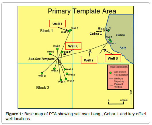
Figure 1: Base map of PTA showing salt over hang , Cobra 1 and key offset well locations.
The major geologic structure in the PTA is interbedded sandstone and shale. These sediments are Miocene to Pleistocene in age. A large salt intrusion lies in Block 2 roughly 4000 ft below the seafloor. The edge of this salt diapir trends northwest-southeast and spans over the entire eastern half of Block 2.
A complete offset well historical analysis was conducted for each well in the PTA. Drilling problems related to incorrect mud weights for the chosen key offset wells (Well 1, Well i, Well 3, and Well C) were among the most severe in the field. While Well 1 was relatively trouble free, kicks and lost circulation events were experienced in wells i, 3, and C. Lost circulation events due to depleted reservoir sands were encountered by Well C, which drilled four bypasses, and well 3, which was Plugged and Abandoned (P&A) before reaching Target Depth (TD). Wells i and 3 endured wellbore stability issues along with lost circulation as they approached the salt overhang.
Pore pressure
One main cause of over pressured formations is known as the compaction phenomena [1]. The relationship between compaction and overburden stress can be demonstrated by the classic fluid filled cylinder example [2]. Overburden force (S) is supported by the upward force of the rock matrix (σ), also known as effective stress, and the fluid pressure (p). Thus, yielding Equation. (1) expressed as [3]:
 (1)
(1)
Overburden increases with burial, resulting in an increase in compaction with depth. As long as the pore-fluid is free to escape with further compaction, the formation will remain normally pressured, because the freely moving pore-fluid can be considered as one large column of water. However, if the fluid is restricted from leaving the pore space it will begin to support a larger portion of the overburden load as burial continues, resulting in a decrease in effective stress gradient and an increase in pore pressure gradient with depth. This phenomenon is known as “Under compaction,” and commonly occurs within thick sections of impermeable shale’s and in areas of rapid deposition, such as the Mississippi River Delta [3]. Furthermore, smaller effective stress and pore pressure increase can be created due to unloading caused by formation uplift [4]. Therefore, it is critical to establish a relationship between effective stress and available transit time.
While many consider under compaction to be the primary source for abnormal pressures, overpressure can also be caused by other mechanisms such as fluid expansion. This occurs through heating, hydrocarbon maturation, charging from other zones, and expansion of intergranular water during clay diagnosis. If the rock matrix constrains the escape of pore fluids during any of these processes, pore pressure will build in the formation as the fluid attempts to increase in volume while porosity remains constant [5].
Petrophysical approach for pore pressure prediction
The process of predicting shale pore pressures by use of petrophysical logs was pioneered by Hottman and Johnson. Applying the principle first presented by Hubert and Rubey that for a given porosity (?) in a clay formation, there exists a maximum value of effective stress which the clay matrix can support without further compaction. Ultimately, this means that if fluid pressure is abnormal, then the porosity within that formation will be abnormally high, or “under compacted,” for a given burial depth [6].
An empirical approach was taken when determining relationships between petrophysical data and porosity [6]. By observing “Normal Compaction Trends” in interval transit time and resistivity log measurements with depth, they were able to develop empirical relationships based on data point deviations from the Normal Compaction Trend Line (NCTL) that could predict the location and magnitude of abnormal formation pressures along a wellbore trajectory.
Others [5,7] have built upon the petrophysical pore pressure prediction approach by developing empirical equations based on Equation. (1) that transform the porosity trends to pore pressure by use of the NCTL. These applications can be successful if there is a relationship between porosity and pore pressure, but in situations where this is not true (i.e. thermal expansion) the porosity trend application can yield erroneous results. New approaches for predicting pore pressure from well logs were also presented by [8], where empirical methods for abnormal pore pressure prediction were adopted to provide a much easier way to handle normal compaction trend lines.
Seismic interval velocity approach to pore pressure prediction
Some of the first attempts to predict pore pressure from the use of reflection seismograph data were made in 1968 [9]. Pennebaker first found average velocity for each reflective horizon in a given survey. By using commonly accepted geophysical relationships, the average velocities were converted to interval travel times. The interval travel times were then plotted verse depth, and much like the Hottman and Johnson method, overlays were made which would predict pore pressure magnitudes based on empirical relationships between the travel time data and their departure from a normal compaction trend line [9].
Since then, advances in geophysical data processing and velocity analysis methods have made predicting pore pressure from velocity seismic data the most commonly accepted practice for modern pore pressure projections. Once the velocity data is processed and converted into interval transit times along a proposed wellbore trajectory, the application of any acoustic log pore pressure prediction method, such as Eaton or Bowers, would output estimated magnitudes for geopressure.
There are, however, issues with the seismic interval velocity approach. Rock velocities are dependent on many factors: lithology, porosity, fluid saturation, confining stress, pore structure, temperature, pore fluid type, clay content, dipping horizons, and cementation [10]. The dependency on multiple parameters increases the uncertainty of relating a change in interval velocity to a change in pore pressure.
For this study, the influence of lithology on interval velocities is the dominant issue. Due to the irregular shape and complex structure of a salt diapir, any seismic velocity analysis or seismic processing carried out in proximity to it will likely yield erroneous results, at least to some degree [11]. The negative effects of salt on seismic velocity analysis are well known, and it is outside of the scope of this paper to discuss these issues in detail.
Seismic frequency approach to pore pressure prediction
Seismic surveys will provide both velocity and frequency data. The quality factor (Q) is a term used to describe the attenuation of seismic signal energy as it propagates through the subsurface. A high Q is consistent with a rock that transmits the seismic signal well, and low Q describes a rock that does this poorly. For example, a bell that is of very high quality will ring for much longer and present a greater bandwidth of frequencies than a bell that has an imperfection such as a crack. The first bell has a greater Q factor.
The Q factor has been suggested as a tool for pore pressure prediction [12]. Multiple studies [13-17] have shown that when pore pressure is applied to core samples, and a seismic wave is passed through the sample, Q factor decreases with decreasing effective stress. One study [13] compared the response of Q to increasing pore pressure with confining pressure remaining constant to the response of rock velocity under the same conditions (Figures 2 and 3). With a decrease of approximately 150%, Q was much more sensitive to pore pressure increase in these conditions which resemble pore pressure increase due to thermal expansion and not under compaction. Velocity showed a decrease of only 5%. This adds to argument that rock velocity is more dependent on porosity than actual effective stress magnitude [13].
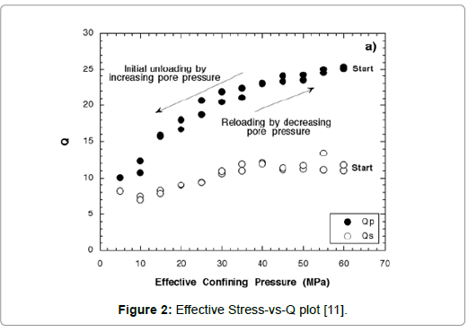
Figure 2: Effective Stress-vs-Q plot [11].
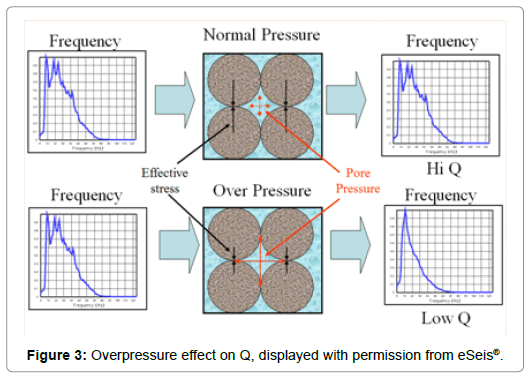
Figure 3: Overpressure effect on Q, displayed with permission from eSeis®.
The Q factor is not dependent on porosity or lithology, but is influenced by the grain-to-grain contact that is controlled by effective stress. Grains within rock samples will separate as fluid pressure increases (Figure 4). Analogous to a crack in a bell, this creates a less continuous medium for the seismic wave to travel through, thus, creating a decrease in Q. By the use of frequency data from seismic survey, Q can be determined at each depth and abnormal pressure zones can be located [12].
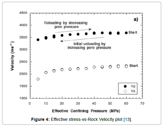
Figure 4: Effective stress-vs-Rock Velocity plot [13].
It is a universally accepted geophysical principle that seismic frequencies will decrease with depth; therefore, when average frequencies are plotted with depth, they will show a normal decreasing trend.
 (2)
(2)
Equation. (2) shows the relationship between Q, the total seismic energy per cycle (E), and the change in energy per cycle (ΔE). The average frequency can correspond to E and the change in frequency corresponds to ΔE. The greater drop in frequency, the lower Q will be for that interval, therefore, lower pore pressure [12].
This method is a very powerful tool and poses drastic advantages over the velocity based geopressure prediction methods. For example, if an under compacted, abnormally pressured formation is uplifted to a shallower depth, it may now have a porosity that is consistent with the surrounding normally pressured formations at that same depth. If the interval velocity approach is applied, this abnormally pressured zone would likely bypass detection. The frequency based method does not take into account porosity. It is a direct measurement of effective stress, and the abnormally pressured formation would be detected since the effective stress within it would be lower than the surrounding horizons.
Sand pore pressure prediction
There are currently no methods for predicting pore pressure in sand formations by using petrophysical or seismic methods. Sand pore pressures are usually obtained by wireline pressure tests or build-up tests, which are carried out after a well is completed. Pore pressure in sand can be predicted by implementing well-known fluid mechanics applications in what is referred to as the centroidal effect [16].
For dipping sand formations that have good hydraulic continuity, Equation (3) can be used to predict the pressure in that sand (ps) at a proposed well location if the pore-fluid pressure gradient (Δpf / D), sand pressure in reference offset well (po), and elevation change of that horizon between the two locations (Δz) are known [18]:
 (3)
(3)
The use of a fluid gradient and elevation change can be used to predict the pressure at each elevation within that sand; therefore, depending on the orientation of the dipping sand bed, the sand pore pressure Equivalent Mud weight (EMW) could be higher or lower than that of the surrounding shale formations [19].
Rock failure
Like all other materials, rocks can either fail under compression or tensile stresses (Figure 5). In order to optimize drilling operations and wellbore stability, it is important to know the Unconfined Compressive Strength (UCS) and tensile strength (To) for all formations to be encountered by a proposed wellbore trajectory. If these, along with the orientation and magnitudes of the three principle stresses (σ1, σ2 and σ3), mud pressure (pi) and pore pressure (p), are known, then the mud weight window can be determined so that the wellbore does not fail in tension (lost circulation) or in compression (breakout or collapse hole).
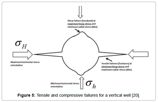
Figure 5: Tensile and compressive failures for a vertical well [20].
By implementing the concept displayed in figure 5 and applying the understanding that tensile fractures occur when σθθ(0°) = -To, the equation for determining the maximum mud pressure in vertical wells before formation tensile fractures occur (pimax) is expressed as:
 (4)
(4)
where σh is minimum horizontal stress, σH is maximum horizontal stress [17].
Predicting shear and tensile fracture pressure
The widely accepted assumption that is made for predicting pimax, or fracture pressure (pf), is that the wellbore will already contain fractures, therefore the To term goes to zero. This simplifies the process by eliminating the need to know every formation’s tensile strength prior to drilling a well.
A direct measurement of fracture pressure at the wellbore can be determined by performing a Leak-Off Test (LOT). LOT data can be misleading if the test is conducted in formations that have excessively higher or lower tensile strength than the formation averages along the wellbore. It is important to keep this in mind when estimating fracture pressures [20-22].
Equation (5) [23] is used as the basis of many fracture pressure prediction methods:
 (5)
(5)
where K is the effective stress ratio and can be expressed as [22].
 (6)
(6)
Various methods for predicting fracture pressure present different approaches on the derivation of K [24,25].
The Mohr-Coulomb failure criterion is often used when determining the shear failure gradient for a well [26]. The Modified Lade Criterion can also be used to determine the shear failure gradient. It differs from Mohr-Coulomb in that it accounts for the influence of all three principle stresses on rock strength, rather than only the minimum and maximum stresses utilized by Mohr-Coulomb [27]. For a more extensive explanation of the Modified Lade Criterion, please see reference [28].
In addition to effect of principle stresses and rock strength, existence of bedding planes and pre-existing fractures can significantly affect borehole stability situation around the wellbore. It is recommended to predict failure gradient in weak planes in order to model wellbore failure in those planes [29].
Effects of depletion on fracture gradient
Generally, when production takes place in a reservoir formation the pore pressure will decrease with volume removal, leaving the overburden stress increasingly supported by the rock matrix, and thus, increasing effective stress [30]. The gravitational loading on the formation matrix will cause a change in horizontal stress while overburden remains constant for an infinite horizontal reservoir. The relationship between pore pressure depletion and horizontal effective stress, assuming no lateral strain, is given by:
 (7)
(7)
where α is Biot’s coefficient and υ is Poisson’s Ratio [31]. Since Δp is negative during depletion, the change in horizontal effective stress will also be negative, meaning that the fracture pressure for the rock will decrease with depletion (Equation (7)).
Effects of salt on stress orientations
When a salt diapir moves up through the formations, it exerts force outward in all directions, which will cause localized changes in the orientation of the principle stresses [32]. It is common directional drilling practice to drill parallel to the minimum horizontal stress if the well is within a normal fault regime, as this orientation gives the wellbore maximum stability. The stress regime surrounding a salt diapir could resemble one consistent with trust faulting, where:
If a well is being drilled in an orientation that is stable for a normal faulting regime and comes in close proximity to a salt diapir, then that wellbore could become unstable and more susceptible to collapsed hole, breakout, or lost circulation [32].
In order to construct a mud weight window for the proposed well, those of key offset wells must be developed first. Mud weight windows for previously drilled wells are produced by the implementation of the following key calibration parameters:
• Available petrophysical data for deriving overburden gradient, pore-pressure gradient, tensile fracture gradient, and shear failure gradient curves
• Mud weights used
• NPT events due to incorrect mud weight
• Measured pressures from LOT and MDTs/RFTs
• Geologic setting
Given the location of the proposed well (Figure 1), the mud weight windows used for calibration will be from wells 1, i, 3, and C.
The estimated pore-pressure, tensile fracture gradient, and shear failure gradient curves will be generated based on the equations, suggested constants, and empirical relationships provided by the literature. Since certain methods are more applicable to certain locations or wells than others, multiple methods to produce each curve type will be applied to increase the probability of correct window estimation. The application of seismic interval velocity and frequency based pore pressure prediction will be completed for each key offset wells and the proposed well
Petrophysical pore pressure gradient
The first step in any mud window prediction is to determine the overburden gradient. This is usually done by use of the bulk-density log [6].
Since the petrophysical methods for predicting pore pressure are based on shale resistivity and acoustic data, the “clean shale” formations encountered by the wellbore must be located. This is done by use of the gamma ray log. The formations that have the highest API reading relative to the surrounding formations will be the considered clean shale’s. Once the clean shale’s have been located, the acoustic and resistivity values at the corresponding vertical depth will be indicated. From that point the resistivity and acoustic and acoustic methods will be used to transform the porosity trends to pore pressure. For a more detailed explanation of how these methods are applied, please see references [5,7].
The “centroid effect” principle will be applied for pore pressure prediction in known sand formations at the proposed wellbore trajectory.
Tensile fracture gradient
Tensile fracture gradients will be determined by applying both Matthews and Kelly’s and Daine’s methods. For a more in-depth discussion of each method please see references [24,25]. For Daine’s method, Poisson Ratio values can be determined from Equation (9) [33]:
 (8)
(8)
where DTS is shear wave transit time and DTC is compression wave transit time. This data is not available for Well C. The pore pressure curve chosen to include in each fracture gradient derivation will be the best performing petrophysically based pore pressure curve for a given well.
For wells 3 and C, the methods described in section 3.8 will be applied to predict the reduced tensile fracture gradient due to depletion.
Shear failure gradient
The implementation of both Mohr-Coulomb and Modified Lade Criterion will be used to determine two different shear failure stress gradients [26,28]. Maximum horizontal stress can be determined by the empirical relationship displayed in Equation (9):
 (9)
(9)
where β is a tectonic stress parameter. The formation’s rock strength properties can be found by using Equations. (10), and (11) [34]:
 (10)
(10)
 (11)
(11)
where ? is friction angle, So is cohesive strength, and Vp is compressional wave velocity. The azimuth for maximum horizontal stress for Well 1 will be assumed to be 075° based on break-out orientations in caliper data from offset wells. In order to account for the effects of the salt diapir on the wells drilled towards it, the maximum horizontal stress orientation for Wells i and 3 is assumed to be parallel to the wellbore azimuths. This assumption implies that the salt intrusion is likely applying pressure outwards from itself in all directions.
Interval velocity based seismic pore pressure prediction approach
In order to use any seismic prediction method, velocity or frequency, the seismic data must be processed in a way that fits the criteria for pore pressure prediction. Most seismic data is processed to enhance events for structural analysis, which in most cases does not cater to the intricate velocity analysis that is performed while processing seismic for geopressure studies. It is vital to use the interval velocities (VINT) and not the stacking velocities (VNMO) when conducting pore pressure work from seismic velocities. Detailing the procedures used to derive the interval velocities for pore pressure prediction goes beyond the scope of this paper. For a more comprehensive study of these methods please see references [10,35,36].
Once the seismic data is processed according to standards acceptable for pore pressure prediction, the interval velocities can be extracted along the path of a given wellbore. The velocities are then converted to interval transit times and calibrated to the acoustic log data used for the petrophysical pore pressure prediction. This is a common approach when applying any seismic velocity pore pressure prediction technique. The Eaton (1975) method was applied for pore pressure transform in this study [7].
Frequency based seismic pore pressure prediction approach
Just as in interval velocity methods, much care has to be taken in the smoothing steps in the seismic processing procedure to mitigate erroneous average frequencies due to noise. These steps are not as tedious as those required for proper interval velocity analysis, and the frequency based method is not as sensitive to factors such as noise as interval velocities are to factors such as lithology and structure.
The average seismic frequencies can be extracted along each wellbore path and plotted with depth. The process is now very similar to acoustic or resistivity prediction methods. There is a normal, steadily decreasing trend for frequency and points where frequency is lower than the normal trend. A line analogous to a NCTL and an Eaton-type empirical relationship can be applied to transform the frequencies to pore pressure magnitudes. This process is known as the Q-Based method. For a more comprehensive understanding of this process please see reference [12].
Determining mud window at proposed well
Special care has to be taken when projecting petro physically derived information from well-specific locations to proposed well locations. All the corresponding data sets must first be compared to gain an understanding of their consistency. Datasets for pore pressure magnitudes can vary even over short distances depending on many factors, but since the well locations are likely in the same depositional environment the NCTLs for a group of wells in close proximity should be relatively consistent. For this same reason, the overburden gradients should also be consistent assuming no major changes in water depth. Salt can create inconsistencies in both NCTL and overburden. It is also best practice to consider worst-case scenario situations when designing a mud weight window or any other aspect of a drilling operation.
In order to determine what information is most appropriate to project to the proposed location, it is best practice to implement the use of geophysical cross sections. This, along with other geologic maps, will help determine similarities in the subsurface between wells. Quality of data is also very important. Wells that have more reliable data will take priority over those that may have questionable borehole measurements.
Data availability may also be factor. In some situations, such as this study, there may be only one offset well that reached the same vertical depth as the proposed well. Since that will be the only data for formations beyond the depths of other offset wells, then data from the deepest offset well must be used for that section in the proposed well.
Mud weight window curves have been produced for each key offset well: (1) Well 1, (2) Well i, (3) Well 3, and (4) Well C (Figures 6-9). These curves were plotted within the requested constants and procedures directed by the literature and methodology presented herein. Accuracy of the outputs was based on agreement between a curve and the calibration parameters listed in section 4.0. Acoustic logbased pore pressure prediction methods and shear failure gradients were not produced for Well C due to the lack of acoustic data.
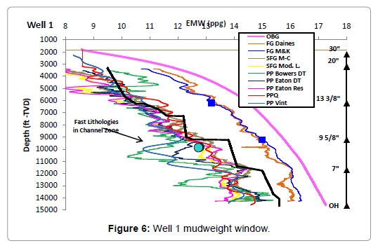
Figure 6: Well 1 mudweight window.
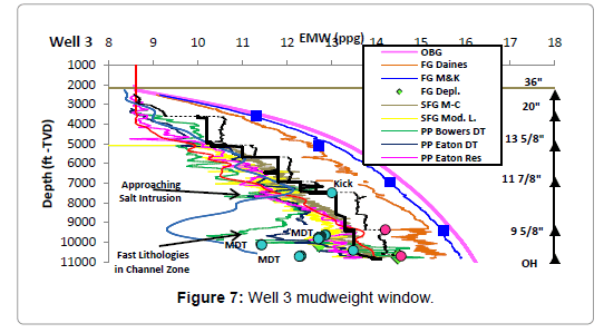
Figure 7: Well 3 mudweight window.
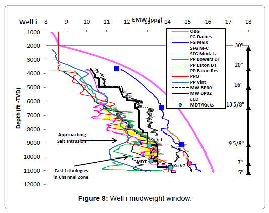
Figure 8: Well i mudweight window.
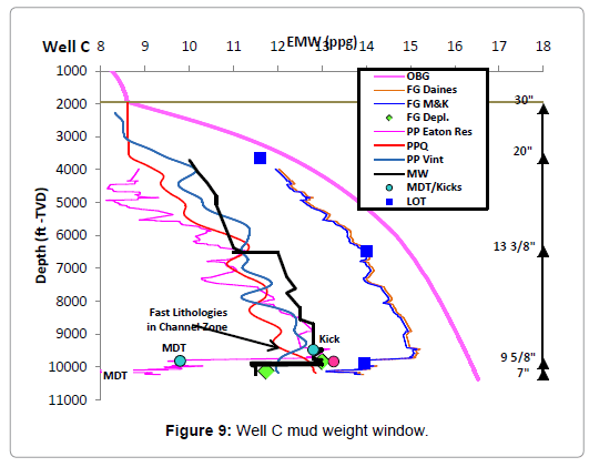
Figure 9: Well C mud weight window.
A new mud weight window was developed for the proposed well location based on the outputs from key offset wells and the methods presented in this paper. The seismic based pore pressure curves were then compared to the petrophysical output for the new well location.
Key offset well mud weight windows
In order to gain a more complete understanding of the subsurface environment, it was necessary to produce mud weight windows for each key offset well using multiple methods to derive each curve type (pore pressure, fracture, and shear failure gradients). Comparing the accuracy of each curve method to a given well and between wells will strengthen the approach to designing a mud weight window for the proposed Cobra 1 well.
Overall, the Eaton resistivity method was the most accurate petrophysically based pore pressure prediction method in this field. (Figures 6-9) will show that the Eaton resistivity method was most consistent at adhering to the calibration parameters in each well, with its best performance perhaps in Well C where it accurately predicted the depleted reservoir pressures (Figure 9). The fact that depletion was detected by a shale-based pore pressure prediction method is likely due to a phenomenon known as shale dewatering, which occurs when severe depletion has taken place in reservoir sands to the point where the shale zones actually begin to deplete also.
The stark influence of lithology on rock velocities can be seen in each well. Starting with Well 1 (Figure 6), the decrease in pore pressure shown in both acoustic log methods and the seismic interval velocity method is an indication of a fast lithology channel zone around 9500 ft to 11,000 ft TVD. This well is not near the salt diapir, so the increased velocities are likely due to a sandy channel zone, where the faster rock velocities are dominating the velocity measurements taken by both the reflection seismograph and acoustic logging instruments.
Though not as pronounced as in Well 1, this effect is evident in the interval velocity output for Well C which is also not near salt (Figure 9).
This hypothesis is supported by low pore pressure/fast rock velocities indicated by the acoustic prediction methods for Wells i and 3 at the same depth interval (Figures 7 and 8). The close vicinity to salt, while likely the cause for low pore pressure/fast rock velocities seen in the seismic interval velocity method, does not affect acoustic measurements taken in the borehole.
Shale points in each well were chosen on a conservative basis, but the shale formations in this channel zone are very sandy, resulting in lower interval transit times. This statement is reinforced by the fact that the acoustic methods (more so the Eaton acoustic method for this field) follow the mud weights used for each well relatively closely at the depths outside the fast channel zone interval. The Eaton resistivity based method being in high agreement to calibration parameters within the channel interval while using the identical shale points to produce its curve lends further support to this claim. These results make evident the prioritization of factors such as lithology and lithologic characteristics over effective stress when it comes to rock velocities.
While the seismic interval velocity pore pressure prediction method was greatly influenced by the presence of salt and fast channel zone velocities, the Q-Based (denoted as PPQ) method appeared to be unaffected by both in each of the key offset wells. The Q-Based curve matched closely to the calibration parameters for each well. Since the seismic data used for this study was collected before most of the production had taken place, the Q-Based method did not successfully indicate the depleted pressures seen in Well C.
The kick event in Well 3 was likely due to a penetrated seal in hydraulically charged sand (Figure 7). By applying the mud weight used in Well i at this sand horizon (12.6 ppg) along with difference in elevation for this sand between wells (150 ft), the centroid principle would yield an estimated pore pressure of 12.9 ppg, assuming the pore fluid is gas. The kick was measured to be 13.0 ppg, and the kick fluid was gas. The centroid effect phenomena would explain why this measured kick pressure is so much higher than any of the derived shale pore pressures at the depth of interest.
Both fracture gradient methods were relatively accurate in correlating to well events and LOTs. Both methods would predict the lost circulation event in Well i at around 10,500’ TVD (Figure 8). The Daines method was successful if correlating to the precise point where the ECD for Well 3 crossed a weak-lithology fracture gradient and endured its first lost circulation event at 9360 ft TVD (Figure 7). The method applied for depleted fracture gradient was accurate for both Wells 3 and C (Figures 7 and 9).
The Mohr-Coulomb method for shear failure gradient appeared to be more accurate than the Modified Lade in calibrating to well events. In both Wells i and 3 the Mohr-Coulomb shear failure gradient curve crosses the mud weight lines used for those wells in the hole sections where the wellbore was near or sub salt (Figures 7 and 8). This is consistent with the poor whole conditions endured by both wells at these intervals.
Development of mud weight window for proposed well
The proposed well (Cobra 1) will be drilled to a TD of 14,000 ft TVD and traverse under the salt diapir overhang (Figure 1). The proposed mud weight window for this well has been developed using information from the key offset wells and applying the concepts expressed in section 4.6 (Figure 10). This information has allowed for a high-confidence mud weight and casing depth design for Cobra 1.
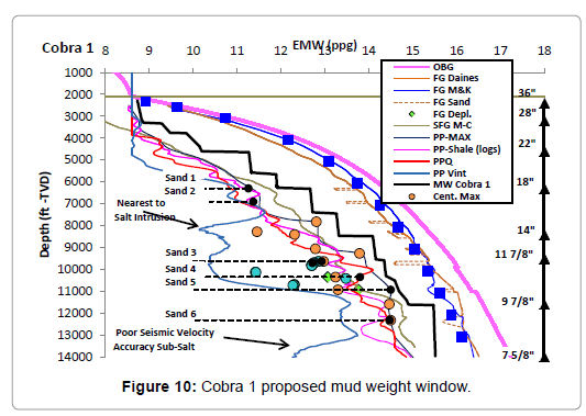
Figure 10: Cobra 1 proposed mud weight window.
Developing the overburden gradient for the new location involved using information from Well 1 and Well 3. Due to the high consistency between the bulk density logs for these wells, the data was spliced together and used to output the overburden gradient at the proposed well.
After extensive study of the subsurface structure and collaboration with the geologist, the maximum expected shale pore pressure curve was based on the maximum values between the Eaton resistivity curve from Well 3 and Eaton resistivity and acoustic curves from Well 1 at a given depth.
The expected sand pressures based on centroid effect were then plotted for the sands that had offset well pressure measurements. Change in elevation for sand horizons between wells was determined by use of seismic cross sections. For worst-case scenario projections, the greatest elevation difference found between any given offset well and Cobra 1 for particular sand was used. A gas gradient of 0.114 psi/ft was applied. The expected pressures in the target sands were supplied by the reservoir engineer.
The determination of K for the Matthews and Kelly fracture gradient was made by normalizing all of the LOT data from the offsets to the water depth at Cobra 1, then plotting the estimated pf values based on a best fit equation. A constant of 0.43 was used for Poisson’s Ratio in the Daines method, as this value matched best with the normalized LOT curve and was close to the average Poisson’s Ratio seen in the offset wells. The Poisson Ratio seen in corresponding sand horizons in offset wells was applied to produce the sand fracture gradient.
Although it is not predicted, the depleted sand fracture gradient was found in the target sand intervals for the worst-case scenario condition. To stay constant with the sands in Well 3, a Poisson’s Ratio of 0.4 was applied for that calculation. These are considered to be accurate do to the highly consistent results found in Wells 3 and C upon application of Equation. (7).
The Mohr-Coulomb method was applied for the shear failure gradient curve, as it showed more accurate results in the key offset wells. The azimuth of σH was changed to 85° due to the anticipated effects from the salt diapir. Since there is no site-specific acoustic data for this proposed well, a splice between the seismic interval velocities at the depths not near salt and key offset well acoustic data for intervals near salt was used to determine friction angle and cohesive strength. The authors warn, due to the lack of valid interval velocity data in the near salt interval for this proposed well, this curve may not be a true representation of the shear failure gradient at Cobra 1. This curve is consistent in trend and magnitude with those of Wells i and 3.
Comparison to seismic-produced curves
When overlaid on the mud weight window derived from key offset well information, it is clear that there is high consistency between the Q-Based curve and the petrophysically derived pore pressure curve (Figure 10). These curves would not be expected to match exactly, since the Q-Based method is site specific to Cobra 1 and the petrophysically based curve is projected from offset well locations.
The Q-Based curve does indicate higher pore pressure than the petrophysically based curve at 10,000 ft TVD, which causes a minor shift in the maximum expected pore pressure curve. The increased pore pressure indicated by the Q-Based curve at this depth could be the result of trapped pore fluid being sealed against the salt face and pressurized from a combination of pore fluid migration from below and the force of the salt pushing out against the formations.
The interval velocity curve is relatively consistent with the other well information until the projected wellbore is within 1000 lateral feet of the salt intrusion at approximately 7000 ft TVD. Below this point, the effect of salt on seismic interval velocity is evident, as the pore pressure predictions begin to be much lower than what was seen in the mud weights for key offset wells.
The powerful advantage that the Q-Based method has over the interval velocity method in subsurface environments such as those presented in this study can best be observed when given the hypothetical situation that this proposed well location is that of an exploration well. In this situation, seismic methods are most often the only available means for reliable pore pressure prediction. (Figure 11) shows such a condition, where all the information that is available for a development well, such as MDTs, LOTs, derived pore pressure curves from nearby offsets, and estimated centroid pressures, has been removed.
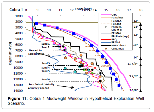
Figure 11: Cobra 1 Mudweight Window in Hypothetical Exploration Well Scenario.
The petrophysically derived pore pressure curve has been dotted to show the high agreement between it and the Q-Based method in this near-salt location. Planning a mud program and plotting casing depths based on the Q-Based curve would not yield results that are drastically different than those for the development well situation, but using the interval velocity based curve in this environment could have obvious negative results.
A systematic approach to mud weight window design for a proposed well has been demonstrated. A historical analysis and petrophysically based methods were applied at each key offset well to assess the subsurface environment. That information was applied to define the mud weight window for the Cobra 1 well. For the first time, seismic interval velocity and the Q-Based pore pressure prediction methods were compared. Their accuracy was based on conformance to calibration parameters in the key offset wells and the final proposed well mud weight window output. This study resulted in the following conclusions:
• The Q-Based seismic pore pressure method performed with greater accuracy than the interval velocity based method in each key offset well and the proposed well.
• The interval velocity method yielded erroneous results in a fastrock- velocity channel zone and the near salt proximity environments, whereas the Q-Based method appeared unaffected by either of these factors.
• The application of multiple methods for deriving each mud weight window curve allowed for increased confidence in mud weight and casing depth design at a proposed well location.
• Comparing curve outputs to the calibration parameters at the offset wells and to corresponding outputs between wells resulted in the indication of key geologic features.
The items presented in this study can be applied to any proposed well mud weight window generation. Most of the commonly used methods are based on empirical relationships or trends that may support certain subsurface environments over others. Exercising techniques that reduce these uncertainties, such as the use of multiple methods to generate a given curve type, is highly recommended. Ultimately, accuracy of mud weight window development for an existing or proposed well will be a function of data quality and sitespecific geologic understanding.
The authors would like to thank Stone Energy Corp. for providing the resources and support that made this project possible. Acknowledgments are also given to eSeis for their support and permission to present the Q-Based theoretical basis, methodology, and output in this study.