Journal of Geology & Geophysics
Open Access
ISSN: 2381-8719
ISSN: 2381-8719
Research Article - (2015) Volume 4, Issue 5
Lithofacies succession in Chaibasa-Noamundi basin of the Proterozoic Kolhan Group, Jharkhand has been studied statistically using modified Markov chain model and Entropy function. The lithofacies analysis based on the field descriptions, petrographic investigation, and their vertical packaging has been done for assessing the sediment depositional framework and the environment of deposition. Six lithofacies arranged, in two genetic sequences, have been recognized within the succession. The result of Markov chain analysis indicates that the deposition of the lithofacies is non-markovian process and represents asymmetric fining-upward non-cyclic deposition. The chi-square test has been done to test for the hypotheses of lithofacies transition at confidence level of 95%. The entropy analysis has been done to evaluate the randomness of occurrence of lithofacies in a succession. Two types of entropies are related to every state; one is relevant to the Markov matrix expressing the upward transitions (entropy after deposition), and the other, relevant to the matrix expressing the downward transitions (entropy before deposition). The energy regime calculated from the entropy analysis showing maximum randomness, suggests that changing pattern in deposition has been a result of rapid to steady flow. This results a change in the depositional pattern from deltaic to lacustrine deposit and sediment by passing that finally generated non-cyclicity in the sequence.
Keywords: Markov chain analysis; Entropy analysis; Kolhan basin; Cyclicity; Chaibasa-noamundi basin; Lithofacies succession
The Kolhan group lying unconformably above the Singhbhum granite and is preserved as a linear belt extending for 80-100 km with an average width of 10-12 km. It is bounded by the Jagannathpur lavas on the southeast and south and by the faulted Iron Ore Group on its western contact. Saha [1] has divided the Kolhan Group of sediments into four detached sub-basins-Chaibasa-Noamundi basin, Chamakpur- Keonjhargarh basin, Mankarchua basin and Sarapalli- Kamakhyanagar basin.
The complex patterns in lithologic successions are produced as a result of the physical process and random events occurring simultaneously in a given depositional environment. It is therefore required that sedimentary succession to be tested for such cyclic order on an objective and quantitative basis. Due to absence of fossils assemblages, land vegetation and paucity of exposure, it is difficult to interpret depositional environment of Proterozoic Kolhan sequence. In the Chaibasa-Noamundi basin it is observed that there is gross lithological asymmetricity present between various lithofacies. There is marked difference in the sandstone and shale thickness, with shale thickness very high as compared to sandstone. It is difficult to prove in the field time independent depositional relational, if any, between the two sedimentary units as there is absence of unconformity in the sequence. Markov chain analysis was carried out to analyze the order of sequence and transition in the facies lineage. To prove similar cyclic arrangement in the lithofacies in the study area, the Markov property and entropy analysis was applied to test for the presence of order in the sequence of structures or descriptive facies in the Chaibasa-Noamundi Basin.
The present study is based on the outcrop and subsurface data of the Chaibasa-Noamundi basin from seventeen sedimentary logs to find the cyclicity of lithofacies using Markov Chain and Entropy analysis. The aim of this paper is
• To evaluate statistically cyclic character by Markov chain analysis; to compare the cyclicity, if present, in time and space.
• To evaluate the degree of ordering or energy regime of the facies deposition using entropy functions.
• To recognize the broad depositional environment of the basin.
Geological setting and stratigraphic succession
In eastern India, Singhbhum craton is mainly composed of Archean granitoids bounded in the north and east by a Proterozoic mobile belt (Table 1) [1]. Dunn [2] first recognized the Kolhan group of sediment towards the western part of the Singhbhum granite, preserved as a linear belt extending for 80-100 km with an average width of 10-12 km with broad wraps and dome and basin structure (Figure 1).
| Newer Dolerite dykes and sills | ca. 1.6- 0.95 Ga |
| Mayurbhanj Granite | ca. 2.1 Ga |
| Gabbro – anorthosite – ultramafics | - |
| Kolhan Group | ca. 2.1- 2.2 Ga |
| Unconformity | |
| Jagannathpur / Malangtoli and Dhanjori–Simlipal | ca. 2.3 Ga |
| Lavas, Quartzite– Conglomerate (Dhanjori Group) | ca. 2.3 - 2.4 Ga |
| Pelitic and arenaceousmetasediments with mafic sills (Singhbhum Group) | |
| Unconformity | |
| Singhbhum Granite Phase III (SBG B) | ca. 3.1 Ga |
| Epidiorites (intrusives) Iron Ore Group (IOG, volcano sediments | - |
| Unconformity | |
| Singhbhum Granite Phase I and II (SBG A), NilgiriGranite, Bonai Granite | ca. 3.3 Ga |
Table 1: Simplified chronostratigraphic succession for the singhbhum craton, eastern india [1,4].
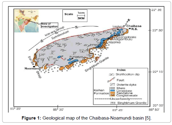
Figure 1: Geological map of the Chaibasa-Noamundi basin [5].
The main basin of Chaibasa-Noamundi extends for about 60 km length with an average width of 10-12 km from Noamundi (85°28’– 22°09’) in the south to Chaibasa (85°48’–22°33’) in the north. The strike of basin is in NNW-SSE direction and low westerly dip of 5 to 10°. The metasedimentary rocks comprising of basal conglomerate, sandstone, limestone and phyllitic shale lie unconformably over the Singhbhum granite in the east and partly over, folded and thrust-faulted, Iron-Ore Group to the west [3]. The sediments have undergone gentle tectonic deformation and very low grade metamorphism [3].
Lithological succession
The major lithounits of Chaibasa-Noamundi basin are Kolhan shale, Kolhan calcareous shale/limestone, Kolhan sandstone, Kolhan conglomerate. The Kolhan Sandstone overlies the granitoids basement with an erosional unconformity often strewn with thin layers and lenses of conglomerates [4]. In all these exposures the minimum thickness attained is 4.57 m while maximum goes upto 7.62 to 9.14 m. The planebedded sandstones are interbedded with minor thin beds and lenses of conglomerates, pebbly sandstones with thin and impersistent layers of shale [3]. The sandstone shows development of antidune/wavy lamination and planar cross stratification. The stratigraphy of chaibasa- Noamundi basin shows very thin sandstone overlain by thick shale deposit represents an asymmetry in vertical basin-fill architecture [4]. The Kolhan Limestone is an impersistent horizon. It is best developed towards SW of Chaibasa, near village Rajanka and Kondoa and N and NW of Jagannathpur.
Six lithofacies has been identified after grouping of lithounits together based on their gross lithologies, primary sedimentary structures, and paleocurrent patterns [5-7]. The architectural elements used in the present study are the sedimentary structures, textures, fabrics of the lithofacies, stratal characteristics and geometrical relationships [8]. The six lithofacies are (a) granular lag facies (GLA), (b) granular sandstone facies (GSD), (c) sheet sandstone facies (SSD), (d) plane laminated sandstone facies (PLSD), (e) rippled sandstone facies (RSD), and (f) thin laminated siltstone-sandstone facies (TLSD) [6,7].
Six lithofacies have been recorded and are described individually as,
1) Granular Lag Facies (GLA): This facies is characterized by the occurrence of laterally impersistent, massive, ungraded and fine matrix supported conglomerate. These conglomerates are mostly immature to sub-mature, and quite similar to the overlying sandstone (Figure 2A).
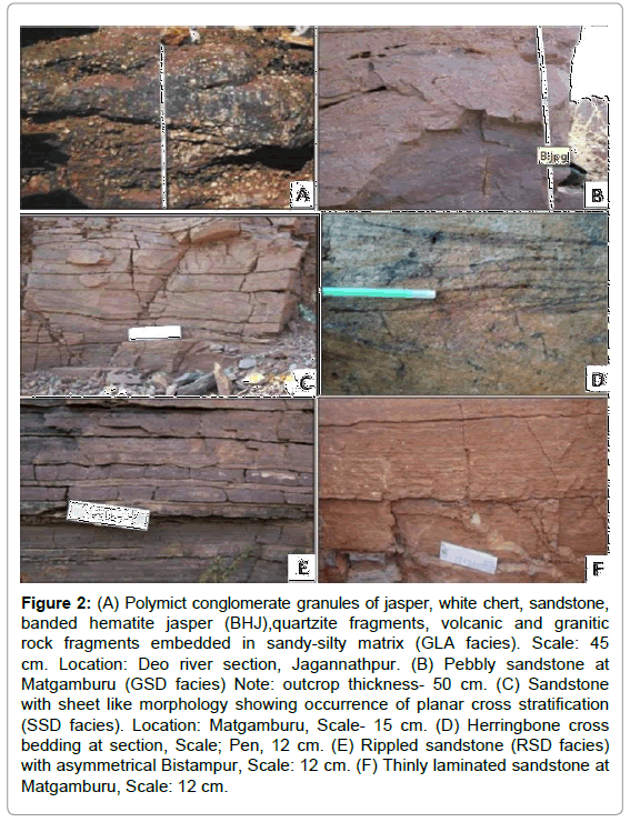
Figure 2: (A) Polymict conglomerate granules of jasper, white chert, sandstone, banded hematite jasper (BHJ),quartzite fragments, volcanic and granitic rock fragments embedded in sandy-silty matrix (GLA facies). Scale: 45 cm. Location: Deo river section, Jagannathpur. (B) Pebbly sandstone at Matgamburu (GSD facies) Note: outcrop thickness- 50 cm. (C) Sandstone with sheet like morphology showing occurrence of planar cross stratification (SSD facies). Location: Matgamburu, Scale- 15 cm. (D) Herringbone cross bedding at section, Scale; Pen, 12 cm. (E) Rippled sandstone (RSD facies) with asymmetrical Bistampur, Scale: 12 cm. (F) Thinly laminated sandstone at Matgamburu, Scale: 12 cm.
2) Granular sandstone facies (GSD): This facies is characterized by moderately to well sorted, moderate clast/matrix ratio. Planar cross-stratification is more commonly found in compare to trough cross- stratification (Figure 2B).
3) Sheet sandstone facies (SSD): The SSD facies is defined by sheets of subarkose-sublithic arenite-quartz arenite, sometimes intercalated with thin laminated siltstone (Figure 2C).
4) Plane laminated sandstone facies (PLSD): The PLSD facies is defined by thick amalgamated well sorted subarkose- sublithic arenite-quartz arenite, with a moderate - high grain: matrix ratio. The sandstone is medium to fine grained. The prominent structures are planar cross bedding, wavy lamination, and washed out/flat top ripples, herringbone cross-bedding and antidunes (Figure 2D).
5) Rippled sandstone facies: This facies is defined by predominance of packages of rippled sandstone with prolific development of both symmetrical and asymmetrical ripples (Figure 2E).
6) Thin laminated sandstone facies: This facies is defined by the rhythmic alternation of sandstone and shale units (Figure 2F), in which sandy layers are thicker than shale layers.
The cyclic sedimentation is wide concept and has application in a wide variety of sedimentary environment [9]. Cyclicity in a sedimentary succession is defined as a series of lithologic units or lithofacies repeated through a succession in a cyclic or rhythmic pattern to some extent. Two types of observable cyclicity may be noteworthy: one in which there exist an order of sequence only; and another in which there is a certain order of repetition along the vertical scale of the sedimentary succession. Which type of cyclicity is to be considered is determined from the geological problem [10]. In this study each “bed” provides a logical unit, therefore, examining cyclicity of a sequence is appropriate, hence it safer to ignore thickness [11].
Structuring data for markov chain
Vertical sequence profile: Seventeen lithological sections were considered for studying the vertical and areal distributions of the lithofacies within the Chaibasa-Noamundi basin.
Nature of Data: The data used in the study is different lithofacies in a vertical sedimentary log sequence coded into finite number of states for the statistical analysis [12]. In this study only six lithofacies are used which are clearly marked in outcrop section as well as in each sedimentary log and this is also done in order to prevent diffusion of transitions between two lithofacies [13].
For the statistical interrelationships between different lithofacies, following six variables were extracted from the seventeen vertical log successions. The six lithofacies variables (descriptive characteristic is in the previous section) and the symbols used to designate them are as:
A- Granular lag facies (GLA),
B- Granular sandstone facies (GSD),
C- Sheet sandstone facies (SSD),
D- Plane laminated sandstone facies (PLSD),
E- Rippled sandstone facies (RSD),
F- Thin laminated sandstone facies (TLSD).
All six states are well represented in each of the seventeen sedimentary logs.
Calculation of frequency count matrix (F): Frequency count matrix is calculated from the vertical sequence profile of sedimentary logs. Since we are using Markov chain which has memory less property i.e. the geologic situation at point (n-1) governs the event that will happen at n. That’s why all seventeen sedimentary logs can be used to calculate matrix F without loss of information. Subsequently, data for all logs are added and matrix is structured at the basin level [14]. Number of transition from facies i to j is represented in row i and column j of matrix F, which signifies number of times state j followed immediately after state I in the sedimentary logs.
The frequency count matrix is structured into embedded Markov chain (definition below) considering only transition of lithologies and not their thickness as stated elsewhere. Since a transition is supposed to occur only when it results in a different lithology, the diagonal elements are all zero’s in the resulting frequency matrix [14].
Analytical procedure
In the present study, the embedded Markov matrix is used for structuring the frequency count matrix (Fij), where i, j is the row and column number respectively. When i=j, zero is present in the matrix, this implies that the transition from one facies to another has only been recorded where there is an abrupt change in the lithofacies. The advantage of the embedded Markov matrix over the regular Markov matrix is that it is used to identify an actual order in facies transition, if present, regardless of the thickness of the individual bed [13].
Transition frequency matrix (F): It is a two dimensional array which records the frequency of the vertical transitions that occur between the different lithofacies in a given stratigraphic succession. The lower facies of each transition couplet are given by the row numbers of the matrix, and the upper facies by the column numbers.
Upward transition probability matrix (P): The upward transition probability matrix calculates the probability of upward transition of lithofacies in a succession and is calculated in the following manner:
Pij=Fij/SRi
Where, SRi is the corresponding row total.
Downward transition probability matrix (Q): Downward transition probability determined by dividing elements of the transition frequency matrix (F) by the corresponding column total, i.e.
Qji=Fij/SCj
Where, SCj is the column total. It calculates the probability of downward transition of lithofacies in a given succession i.e probability of facies i overlain by facies j.
Independent trail matrix (R): This matrix represents the probability of the given transition that occur in a random manner and is given by,
Rij=SCj/(ST – SRi)
Where, ST represents total number of facies transition. The diagonal cells are filled with zeros assuming each transition represent an abrupt change in facies characteristic.
Difference matrix (D): A difference matrix is calculated which highlights those transitions that have a probability of occurrence greater than if the sequence were random. By linking positive values of the difference matrix, a preferred upward path of facies transitions can be constructed which can be interpreted in terms of depositional processes that led to this particular arrangement of facies [15].
Dij=Pij–Rij
A positive value in difference matrix indicates that a particular transition occurs more frequently and a negative value indicates that it occurs less frequently. In difference matrix the values in each rows of the matrix sum to zero. If the values are close to zero, a vertical succession with little or no ‘memory’ indicates independent nature of deposition of facies in a basin.
Expected frequency matrix (E): Expected frequency Matrix represents the expected number of transition from facies i to facies j and is given by
Eij=Rij × SRi
It is necessary to calculate an expected frequency matrix, since chi – square tests should only be applied when the minimum expected frequency in any cell not exceeds 5.
Test of significance: Non-parametric chi-square (χ2) test has been applied to ascertain whether the given sequence has a Markovian ‘memory’ or no memory. To test null hypothesis, chi-square (χ2) values are calculated for vertical successions.
Where, Fij=transition count matrix or observed frequency of elements in the transition count matrix; Eij=Expected frequency matrix; ν=degree of freedom given (n2–2n), where n denotes rank of the matrix.
If the computed values of chi-square exceed the limiting values at the 0.5% significance level suggests the Markovity and cyclic arrangement of facies states.
The concept of entropy to sedimentary successions is applied to determine the degree of random occurrence of lithofacies in the succession [16]. Hattori [16] recognized two types of entropies with respect to each lithological state; one is post–depositional entropy corresponding to matrix P and the other, pre–depositional entropy, corresponding to matrix Q.
Hattori [16] defined Post – depositional entropy with respect to lithofacies state i as
If Ei (post) is equal to zero, implies that facies i is always succeeded by only facies j in the sequence. If Ei (post) is greater than zero, facies i is likely to be overlain by different states.
Hattori [16] defined pre – depositional entropy with respect to state i as
Large value of entropy signifies that facies i occur independent of the adjacent state. Two entropies together form a entropy set for state i, and serve as indicators of the variety of lithological transitions immediately after and before the occurrence of i, respectively [16].
Interrelationships of post Entropy and pre Entropy is used to classify various cyclic patterns into asymmetric, symmetric and random cycles [16]. The values of entropies increase with the number of lithological facies. To eliminate this influence, Normalization of the entropies is done by the following equation:
En=E/Emax,
Where, Emax = -log2(1/(n-1))
Where, En is the normalized entropy, E is either post–depositional or pre–depositional entropy, and Emax is the maximum entropy possible in a system where n state variable operates.
Matrices used to analyze transitions of lithofacies in Chaibasa- Noamundi basin is calculated using method and equations given in the previous section (Table 2 a-g).
| A | B | C | D | E | F | SRi | T-SRi | |
|---|---|---|---|---|---|---|---|---|
| A | 0 | 1 | 0 | 4 | 1 | 0 | 6 | 43 |
| B | 3 | 0 | 3 | 2 | 5 | 2 | 15 | 34 |
| C | 0 | 5 | 0 | 0 | 1 | 1 | 7 | 42 |
| D | 2 | 1 | 2 | 0 | 4 | 0 | 9 | 40 |
| E | 0 | 2 | 0 | 3 | 0 | 0 | 5 | 44 |
| F | 1 | 3 | 0 | 3 | 0 | 0 | 7 | 42 |
| SCj | 6 | 12 | 5 | 12 | 11 | 3 | Total= 49 | |
a) Transition count matrix (F).
| A | B | C | D | E | F | |
|---|---|---|---|---|---|---|
| A | 0 | 0.166 | 0 | 0.666 | 0.166 | 0 |
| B | 0.2 | 0 | 0.2 | 0.133 | 0.333 | 0.133 |
| C | 0 | 0.714 | 0 | 0 | 0.142 | 0.142 |
| D | 0.222 | 0.111 | 0.222 | 0 | 0.444 | 0 |
| E | 0 | 0.4 | 0 | 0.6 | 0 | 0 |
| F | 0.142 | 0.428571 | 0 | 0.428 | 0 | 0 |
b) Upward transition probability matrix (P).
| A | B | C | D | E | F | |
|---|---|---|---|---|---|---|
| A | 0 | 0.5 | 0 | 0.333 | 0 | 0.166 |
| B | 0.0833 | 0 | 0.416 | 0.083 | 0.166 | 0.25 |
| C | 0 | 0.6 | 0 | 0.4 | 0 | 0 |
| D | 0.333 | 0.166 | 0 | 0 | 0.25 | 0.25 |
| E | 0.09 | 0.454 | 0.09 | 0.363 | 0 | 0 |
| F | 0 | 0.666 | 0.333 | 0 | 0 | 0 |
c) Downward transition probability matrix (q).
| A | B | C | D | E | F | |
|---|---|---|---|---|---|---|
| A | 0 | 0.279 | 0.116 | 0.279 | 0.255 | 0.069 |
| B | 0.162 | 0 | 0.135 | 0.324 | 0.297 | 0.081 |
| C | 0.136 | 0.272 | 0 | 0.272 | 0.25 | 0.068 |
| D | 0.162 | 0.324 | 0.135 | 0 | 0.297 | 0.081 |
| E | 0.157 | 0.315 | 0.131 | 0.315 | 0 | 0.078 |
| F | 0.13 | 0.26 | 0.108 | 0.26 | 0.239 | 0 |
d) Independent Trails Probability Matrix (R).
| A | B | C | D | E | F | |
|---|---|---|---|---|---|---|
| A | 0 | -0.112 | -0.116 | 0.387 | -0.089 | -0.069 |
| B | 0.037 | 0 | 0.064 | -0.19 | 0.036 | 0.052 |
| C | -0.136 | 0.441 | 0 | -0.272 | -0.107 | 0.074 |
| D | 0.06 | -0.213 | 0.087 | 0 | 0.147 | -0.081 |
| E | -0.159 | 0.084 | -0.131 | 0.284 | 0 | -0.0789 |
| F | 0.012 | 0.167 | -0.108 | 0.167 | -0.239 | 0 |
e) Difference Matrix (D).
| A | B | C | D | E | F | |
|---|---|---|---|---|---|---|
| A | 0 | 1.674 | 0.697 | 1.674 | 1.534 | 0.418 |
| B | 2.647 | 0 | 2.205 | 4.994 | 4.852 | 1.323 |
| C | 1 | 2 | 0 | 2 | 1.833 | 0.5 |
| D | 1.35 | 2.7 | 1.125 | 0 | 2.475 | 0.675 |
| E | 0.681 | 1.363 | 0.568 | 1.363 | 0 | 0.34 |
| F | 1 | 2 | 0.833 | 2 | 1.833 | 0 |
f) Expected Frequency Matrix (E).
| Test of Equation | Computed value of | Limiting Value at 0.5% significance Level | Degree of freedom |
|---|---|---|---|
| Billingslay | 27.112 | 45.55 | 24 |
g) Test of Significance.
Table 2: (a-g) Matrices used to analyze transitions of lithofacies in the Kolhan Group.
Markov chain analysis
It is important to note that significant facies transitions represent the most probable facies transitions, but not their actual frequency in the studied sedimentary sequences. Matrix of observed facies transitions contains the real frequencies of facies transitions. The highest values of
and the positive entries of
The computed values of chi-square is lower than the limiting values at the 0.5% significance level this means that the null hypothesis is false, suggesting the deposition of sediments is not by Markovian process and non-cyclic arrangement of facies states in Chaibasa-Noamundi basin (Table 2g). The facies relationship diagram is constructed from the difference matrix results (Figure 3) (Table 2f).
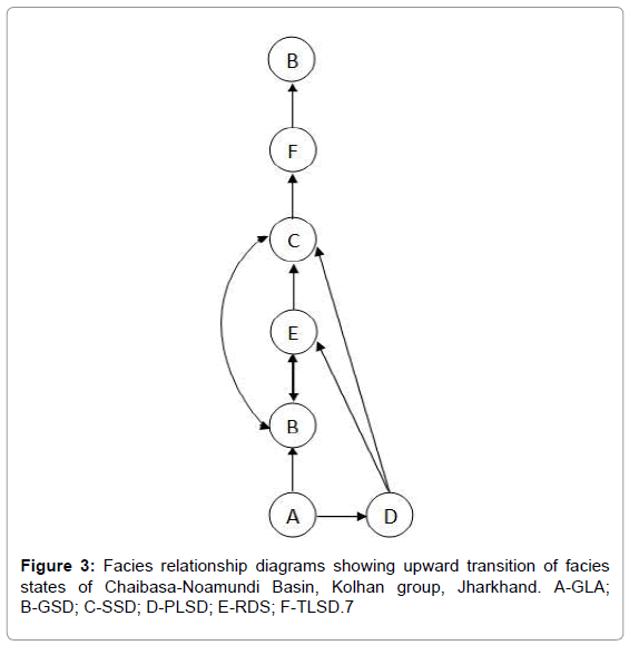
Figure 3: Facies relationship diagrams showing upward transition of facies states of Chaibasa-Noamundi Basin, Kolhan group, Jharkhand. A-GLA; B-GSD; C-SSD; D-PLSD; E-RDS; F-TLSD.7
The preferred upward transition path for the lithofacies is
The transition between is non-Markovian and the lineage is non-repetitive in nature. The obvious aim of this approach was to detect and define cyclic relationships, if any. In the present case the cyclicity is absent or very weak. This information can greatly assist in environmental interpretation.
Entropy analysis
Both Epre and Epost are larger than zero implies all six lithofacies (GLA, GSD, SSD, PLSD, RSD, and TLSD) overlies and also is overlain by more than one state [16]. Epre and Epost are larger in value for GSD and it is deduced that the influx of pebbly sandstone into the Chaibasa- Noamundi basin was the most random event (Table 3). For RSD and PLSD, Epre>Epost. This relation indicates that rippled sandstone could accumulate in a wide variety of depositional environment and exerted a considerably strong influence upon the state selection of its successor.
| EPost | EPre | EnPost | EnPre | |
|---|---|---|---|---|
| A | 0.822 | 0.959 | 0.353 | 0.413 |
| B | 2.232 | 2.054 | 0.961 | 0.885 |
| C | 1.148 | 0.971 | 0.494 | 0.418 |
| D | 1.836 | 1.959 | 0.791 | 0.846 |
| E | 0.971 | 1.159 | 0.418 | 0.499 |
| F | 1.448 | 0.918 | 0.624 | 0.395 |
Table 3: Matrices used to analyze Entropy value of lithofacies in the Kolhan Group.
Large difference in Epre and Epost and with Epre
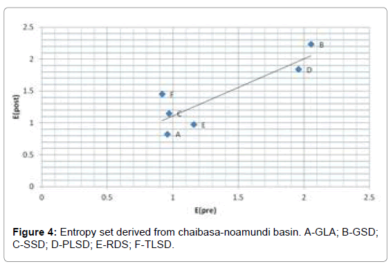
Figure 4: Entropy set derived from chaibasa-noamundi basin. A-GLA; B-GSD; C-SSD; D-PLSD; E-RDS; F-TLSD.
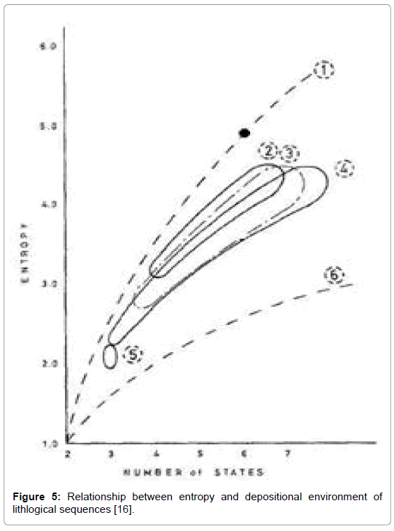
Figure 5: Relationship between entropy and depositional environment of lithlogical sequences [16].
Sediment flow model
In chaibasa-Noamundi basin asymmetric sequence pertains to the sediment bypassing. The thinning-upward sequences represent lacustrine deposits, while the thickening upward sequences represent point bar-sand flat deposits. Variation in layer thickness is suggestive of deposition by unsteady flow in a fluvial regime within the channel. The flow was suddenly impeded, and as a result there was a quick fall in the energy of the solid-fluid system that resulted in rapid deposition. Maximum energy regime of the area deduced from the total entropy analysis suggests that the sequence is not a marine sequence and the overall flow pattern changes from the deltaic environment to lacustrine environment [18]. The granular lag (GLA) and granular sandstone (GSD) facies are a part of shallow braided fluvial plain facies association. These two facies were formed in fluvial channels and bars in braided streams that gradually fanned outwards indicated by the presence of GLA and the GSD facies as the basal layer in the stratigraphic sequence. Trough and planar cross-beddings are common structures developed as a result of the lateral and downstream advance of a midchannel bar that finally coalesced into the adjacent branch channel. High Energy regime can be justified from the field evidence as pebble orientation lacks imbrications implies sudden and rapid deposition. The association of sheet sandstone (SSD), plane laminated sandstone (PLSD), rippled sandstone (RSD), and thin laminated siltstone sandstone (TLSD) facies are typical ephemeral sheet flood facies. Presence of fine - medium grained, well sorted quartz rich sandstones (RSD) frequently interbedded with thin laminated siltstone-sandstone (TLSD) resembling heterolithic facies. The variability of sedimentary structures in the facies associations reflects rapid fluctuations in the supply of sediments. Sedimentary structures, facies relationship and relative abundance of sand and shale in suggest deposition of sediments in different fluvial settings. The transporting mechanisms and dispersal patterns of the Kolhan are complex in nature. Due to small size fine particle travels faster and rapid change in flow leads to sudden deposition leading to thelarge shale thickness as compared to the sandstone. The stratigraphy of Kolhan basin demonstrating very thin sandstone overlain by thick shale represents an asymmetry in vertical basin-fill architecture. Lithofacies variations along strike direction in basal part of shale succession indicate lateral variability among the constituent lithologies within the shale succession. The upper part of the stratigraphy in contrast exhibits widespread and monotonous occurrence of shale. It was proposed that the transgressive Kolhan sequence was deposited in a rift basin setting [7,18].
The Kolhan Group represents the youngest Precambrian stratigraphic unit in Singhbhum geology [1]. The unmetamorphosed, low westerly dipping sedimentary piles lie unconformably over the Singhbhum granite to the east and show a faulted contact with the Iron Ore Group of rocks to the west [1]. The major findings of the study can be summarized as follows:
• The application of the first order Markov Chain analysis on the seventeen vertical sections shows that there is a preferred fining upward transition path in the lithofacies. The operative geological processes were non-Markovian or independent in nature.
• The energy level of the fluid during the entire process shows a considerable fluctuation reflected by the entropy analysis with changing environment of deposition. Variation in layer thickness and asymmetric sequence are suggestive of deposition by unsteady flow in a fluvial regime within the channel. The flow was suddenly impeded, and as a result there was a quick fall in the energy of the solid-fluid system that resulted in rapid deposition.
• It appears that the GLA and the GSD facies represent the channel lag deposits of a braided river and the SSD, RSD, PLSD, and TLSD facies represent the portions of a fining upward sequence complex of a channel bar or possibly the longitudinal bar-transverse barcross- channel bar complex in a fluvial environment. Energy regime related to the total entropy suggests that the shale in distal part of basin is not a marine origin. The flow pattern overall changes from the deltaic environment to lacustrine environment.
The results of this study show that the sedimentary sequence in the Chaibasa-Noamundi basin are non-cyclic, non- Markovian and asymmetric in character.
The authors are grateful to Prof. D Sengupta, Head, Department of Geology and Geophysics, Indian Institute of Technology, Kharagpur, for providing all necessary facilities.