Journal of Geology & Geophysics
Open Access
ISSN: 2381-8719
ISSN: 2381-8719
Research Article - (2015) Volume 4, Issue 2
This paper studies the parallelization of the restarted GMRES solver, GMRES (m), and the block ILU (k) preconditioner on GPUs used in petroleum reservoir simulations. The difficulty is how to accelerate this preconditioner with a variable block size. In this paper, parallel solution techniques for block triangular systems are proposed, which work for matrices with an arbitrary block size. These techniques also work with an arbitrary level k for the block ILU (k) preconditioner. Numerical experiments show that the GPU-based linear solver GMRES (m) is much faster than its CPU version.
Keywords: GMRES solver; Preconditioner; Reservoir simulation; GPU; CPU
The solution of sparse linear systems is the most time-consuming step in running reservoir simulations; over 70% of time is spent on the solution of linear systems derived from the Newton methods [1]. If large highly heterogeneous reservoir models are applied, their linear systems are even harder to solve and require much more simulation time. Hence fast solution techniques are fundamental to large-scale reservoir simulations.
Linear solvers and preconditioners have been studied for decades and various techniques have been developed. Saad et al. developed the GMRES (generalized minimal residual) linear solver, which is a general purpose solver for nonsymmetric linear systems [2,3]. Vinsome designed the ORTHOMIN (orthogonal minimum residual) solver, which was originally developed for reservoir simulations [4]. The BICGSTAB (bi-conjugate gradient stabilized method) solver is also widely applied to reservoir simulations. These Krylov subspace linear solvers are general purpose and can be applied to any kinds of linear systems. When the matrices of linear systems are positive definite, multigrid methods are the most effective, including algebraic multigrid methods and geometrical multigrid methods. It is well-known that the convergence rates of these multigrid solvers are optimal [5-9].
Preconditioners are essential to the success of linear solvers. The incomplete LU factorization (ILU) preconditioners [2,3,10,11] and the incomplete Cholesky factorization preconditioner are the most commonly used preconditioners, which are efficient and easy to implement. The ILU methods are also the base of many advanced preconditioners, such as the domain decomposition methods [12]. For the black oil model, many multi-stage preconditioners [1,13,14] were developed to accelerate the solution of linear systems, such as the constrained pressure residual (CPR) preconditioner [15,16] and the fast auxiliary space preconditioner (FASP) [13]. Chen et al. proposed several CPR-like preconditioners for parallel reservoir simulations on distributed-memory systems [14]. These preconditioners solve a pressure equation using the multigrid solvers and an entire system using the ILU methods.
GPUs (graphics processing units) are extremely fast. Recently, GPU computing becomes more and more popular. However, GPUs have different architectures from CPUs, which means that special data structures and algorithms must be developed to utilize the power of the GPUs. NVIDIA developed a hybrid matrix format HYB for general sparse matrices [17,18]. NVIDIA also provides some fundamental scientific computing libraries, such as FFT (fast Fourier transform) [19], BLAS (basic linear algebra subprograms) [17-19], and sparse Krylov subspace solvers [20]. Saad et al. developed a type of a JAD (jagged diagonal) matrix for GPU computing and its corresponding SpMV (sparse matrix-vector multiplication) algorithm [10,11]. Chen et al. designed a hybrid matrix format, HEC (Hybrid of ELL and CSR), its SpMV algorithm [21], Krylov solvers [14,22-27] and classical AMG solvers [28]. Haase et al. developed a parallel AMG solver for GPU clusters [29]. Bell et al. from NVIDIA investigated fine-grained parallelism of AMG solvers using a single GPU [30]. Bolz, Buatois, Goddeke, Bell, Wang, Brannick, Stone and their collaborators also studied GPU-based parallel algebraic multigrid solvers [31-35]. Naumov [36] and Chen et al. [24] studied parallel triangular solvers for GPUs for point-wise matrices. Typical speedup of the GPU-based triangular solvers is around 2 [11,36]. More details can be found in [11,22-25,31-36].
For reservoir simulations, each grid block has several unknowns, such as pressure, temperature and saturations. If all unknowns in each block are numbered consecutively, the matrix A from the Newton methods has the following structure:
 (1)
(1)
where A is a non-singular matrix, each block Aij (1 ≤ i, j ≤ n) is an m × m matrix, and m is the block size. The same linear system also exists in other applications where more than one equations exist. When m is unity, matrix A is a regular matrix or a regular point-wise matrix; when m>1, it is a block matrix. The block matrix A is equivalent to an nm×nm point-wise matrix. Here the following linear system is studied:
Ax = b, (2)
here b (∈Rnm) is the right-hand side and ×(∈Rnm) is the unknown to be solved. In practice, if A is ill-conditioned, an equivalent sparse linear system is solved:
M-1Ax = M-1b, (3)
Where M is a preconditioner or a left preconditioner. At each iteration, at least one preconditioning system, my = f, must be solved. M may be a point-wise ILU (k) preconditioner, an ILUT preconditioner, a block ILU (k) preconditioner or other pre- conditioners. The Krylov subspace solvers and point-wise ILU preconditioners, such as ILU (k) and ILUT preconditioners, are common methods to solve these linear systems, which are usually effective. However, when the condition number of A is large, the block ILU (k) preconditioner is generally a better choice than the point-wise ILU (k) preconditioner. The point-wise ILU (k) preconditioner and the block ILU (k) preconditioner have been studied and implemented on CPUs by Saad et al. [3].
The block ILU factorization has the form M = LU, where L and U are given as follows:
 (4)
(4)
and
 (5)
(5)
Where Iii is an identity matrix, i = 1, 2, . . , n. The solution of the block ILU preconditioner on CPUs, Mx = b, is the same as the solution of the point-wise ILU preconditioner. The system is written as follows:
Ly = b, U x = y (6)
Equation (6) can be solved by block Gauss elimination in two steps. The first step is to solve the lower triangular system and the second step is to solve the upper triangular system. When parallelizing the GMRES solver and the block ILU (k) preconditioner on GPUs, the implementation of the GMRES solver is straightforward if an efficient sparse matrix-vector multiplication (SpMV) kernel and vector operations are provided. However, the parallelization of the block ILU (k) precon- ditioner is challenging. The reason is that the data on NVIDIA GPUs is stored on the global memory [19], and to achieve optimal efficiency, the data access pattern on GPUs should be coalesced. In addition, when the block size of A is variable, it introduces a difficulty in the design of a parallel block ILU (k) preconditioner on GPUs. In this paper, the point-wise and block ILU (k) preconditioners are studied. The triangular systems from the block ILU (k) factorization are reorganized and a three-step solution algorithm is proposed. The algorithm converts the block triangular systems to point-wise triangular systems; in this case, a unified method is obtained. This three-step algorithm works with any block size. Numerical experiments are performed to test the design of this parallel block ILU (k) preconditioner.
The framework of this paper is as follows: In §2, the GMRES solver and techniques for GPU computing are studied. In §3, the point-wise and block ILU (k) preconditioners are introduced and the solution techniques for the block triangular systems on GPUs are proposed. In §4, numerical experiments are carried to test the performance of the GMRES solver and the block ILU (k) preconditioner.
The GMRES solver is an iterative solution method for nonsymmetric linear systems developed by Saad and Schultz [2,3]. The method approximates a solution by a vector in a Krylov subspace with a minimal residual, where the Krylov subspace is defined by
 (7)
(7)
In practice, the restarted GMRES solver is applied to save memory usage. The algorithm for the restarted GMRES (m) solver with a leftpreconditioner M is given in Algorithm 1.
From Algorithm 1, we can see that all operations except the solution of the preconditioning system are matrix-vector multiplication and vector operations:
y = αAx + βy, (8)
y = αx + βy, (9)
z = αx + βy, (10)
a =
 (12)
(12)
A vector is simply an array and algorithms for vector operations have been studied very well. NVIDIA also provides BLAS operations through the NVIDIA cuBLAS library. However, the sparse matrixvector multiplication (SpMV) operation is much more complicated than the vector operations. The reason is that the NVIDIA GPUs have different architectures from traditional CPUs [19,37] and algorithms that work well on CPUs may not work effectively on GPUs. Special data structures and algorithms for GPUs are required to design. The NVIDIA company developed parallel SpMV algorithms for CSR (compressed sparse row), ELL (EllPack), COO (coordinate) and HYB (Hybrid) matrices. The HYB matrix is a general matrix format for GPU computing, which is a hybrid of an ELL matrix and a COO matrix. Saad et al. designed a parallel SpMV algorithm for the JAD matrix. Here we use a hybrid matrix format HEC, which is shown by Figure 1 [21]. An HEC matrix consists of two parts: an ELL matrix and a CSR matrix. The ELL matrix is regular and each row has the same length. When being stored on GPUs, the matrix is in column-major order. The CSR matrix stores the irregular part of a given matrix. The advantages of the HEC matrix are that it is easy to design a SpMV algorithm and it is also friendly to ILU preconditioners [21,22,24].
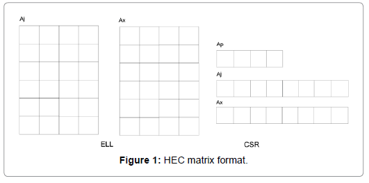
Figure 1: HEC matrix format.
A sparse matrix-vector multiplication kernel [21] is developed as shown in Algorithm 2. The algorithm has two steps. The ELL part is calculated first and then the CSR part is processed. Each GPU thread calculates one row of the given sparse matrix. More details can be found in [21]. If the SpMV kernel and vector operations are implezhe GMRES solver and other Krylov linear solvers can be implemented straightforwardly. In the following sections, we will focus on preconditioners.
In this section, the point-wise and block ILU(k) preconditioners are studied systematically. The point-wise ILU(k) precondi- tioner is introduced first and algorithms for incomplete LU factorization and the solution of triangular systems are presented. Then the block ILU(k) preconditioner is presented. The structure generation of the block ILU(k) preconditioner is based on the point-wise ILU(k) preconditioner. In the end, solution techniques for the block triangular systems are proposed.
The Point-wise ILU(k) preconditioner
Let A be an n × n point-wise matrix, which is equivalent to a block matrix with the unity block size. The matrix is stored by the CSR format matrix, which is demonstrated by Figure 2. The CSR matrix has three arrays, Ap, Aj and Ax. The length of A p is n + 1, which stores the start location of each row in Aj and Ax. For example, Ap(i) is the start location of row i and Ap(i + 1) is the start location of row i + 1. Aj stores column indices of all entries row-by-row and Ax stores values of all entries row-by-row. Usually only non-zero entries are stored in the CSR matrix to save computation and storage. The CSR matrix also defines the sparsity pattern P of matrix A.
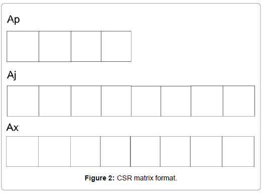
Figure 2: CSR matrix format.
The ILU preconditioner M is defined as M = LU, and the L and the U are
 (13)
(13)
 (14)
(14)
The factorization algorithm of the ILU(0) preconditioner is described by Algorithm 3, in which Aij in L and U is from Algorithm 3, i = 1, 2, . . , n.
The solution for the preconditioning system, Mx = b, is straightforward using Gauss elimination, which is equivalent to system (6). The algorithm is shown in Algorithm 4, which has two steps. The first step is to solve the lower triangular system Ly = b, and the second step is to solve the upper triangular system Ux=y. GPU-based parallel algorithms for the solution of triangular systems have been developed [36].
Regarding as the Algorithm 4, we should mention that the algorithm is highly sequential. Let us take the solution of the lower triangular system, Lx = b, as an example. The ith component of x is solved as follows:
To solve for xi, we must know x1, x2, …, and xi−1, which introduces data dependence and is the bottleneck of parallelization. The solution of the upper triangular system is similar. The level schedule method was introduced to parallelize the solution of triangular systems as shown in Algorithm 7, which will be discussed in detail.
To study a higher level ILU(k) preconditioner, a level for each entry is defined. The initial level for each entry Ai is defined as
 (15)
(15)
The definition means that if one entry exists in the given sparse matrix A, it has a level of zero; otherwise, it has a level of infinity. During the factorization process, the entry Aij is updated by line 5 of the Algorithm 3, and its level is updated by the following formula:
 (16)
(16)
The point-wise ILU (k) is obtained if fill-ins whose levels are less than or equal to k are allowed; the algorithm is shown in Algorithm 5.
Algorithm 5 can also calculate the structure of the point-wise ILU (k) preconditioner by discarding entries whose levels are greater than k. In practice, we calculate its structure first, and then initialize the values of all entries using the original matrix A. The fill-ins have values of zero. At the end, by using the algorithm for the ILU (0) factorization, the point-wise ILU (k) preconditioner is computed. The resulting preconditioning system is solved by Algorithm 4. Algorithms 3 and 5 are from [3] and more details can be found in [3].
Block ILU(k) preconditioner
The block ILU (k) preconditioner is similar to the point-wise ILU (k) preconditioner. The difference is that all operations on the block ILU (k) preconditioner are performed on blocks, which are m × m matrices. The generation of the block ILU (k) preconditioner consists of two steps. The first step is to calculate the structure of the block ILU (k) preconditioner. The second step is to factorize the block matrix.
For the sparse block matrix A, if block Aij exists, then (i, j) belongs to the point-wise matrix P. The P defines the sparsity pattern of the block matrix A. If Algorithm 5 is applied to P, then the structure of the ILU(k) reconditioner for P, Pk , can be obtained. The structure of the block ILU(k) preconditioner for A can be derived by filling zero blocks using Pk . By using the block ILU(0) factorization algorithm, the block ILU(k) factorization can be obtained.
The block ILU(0) factorization is shown in Algorithm 6. All operations on matrix A are matrix operations, such as the inverse of the diagonal matrix Akk , A−1 and the matrix-matrix multiplication Aik×Akj . The lower block triangular matrix L and the upper block triangular matrix U are the same as in (4) and (5). The preconditioning system Mx=b is equivalent to system (6), which can be solved by the forward and backward block Gauss elimination. The implementation on CPUs is straightforward. In the next section, solution techniques on GPUs are proposed.
Solution for block triangular systems on GPUs
When implementing equation (6), a lower triangular linear system, Lx = b, and an upper triangular linear system, U x = b, are required to solve. For a point-wise matrix, the level schedule method [3,11] was adopted to parallelize the solution of triangular linear systems. The idea is to group all unknowns xi into different levels so that the unknowns within the same level can be computed simultaneously [3,11]. For the lower triangular problem, the level of xi (1 ≤ i ≤ n) is defined as
l(i) = 1 + max l( j), for all j such that Lij = 0, i = 1, 2, . . , n, (17)
Where Lij is the (i, j)th entry of L, l(i) is zero initially and n is the number of rows. The level schedule method is described in Algorithm 7. For GPU computing, each level in Algorithm 7 can be parallelized. Parallel triangular solvers for GPUs have been developed [38], which were designed for point-wise matrices. The HEC matrix format [21] was adopted for the parallel triangular solvers, which is demonstrated in Figure 1 [21]. The number of levels in Algorithm 7 depends on the lower triangular matrix L. The ideal case is that there is only one level and the solution process is fully parallelized. The worst case is that the number of levels equals the number of rows; in this case, the solution is completely sequential. The GPUs have the lowest performance.
The level schedule method can also be applied to block matrices. However, since the block size is variable, it is difficult to design algorithms that can match the architectures of GPUs with a variable block size. Here, we reorganize the ILU factorization using three matrices:
M = LD(D-1U ) = LDUs, (18)
where L and U are the same as in (4) and (5) and D is
D = Diag(U11,U22,…,Unn). (19)
 (20)
(20)
The L and Us can be converted to a regular point-wise lower triangular matrix Lt and a point-wise upper triangular matrix Ut . The preconditioning linear system Mx = b is equivalent to the following equation,
Lt DUt x = b, (21)
Which can be solved in three steps:
Lt y = b, z = D−1y, Ut x = z. (22)
Then the block triangular problems are converted to point-wise triangular problems. The linear systems Lty = b and Ut x = z can be solved by the traditional level schedule method, and the system z = D-1y is a matrix-vector multiplication operation. By using the algorithms developed in [38], a parallel solver for block triangular linear systems on GPUs is developed, which works with arbitrary block size. Its algorithm is shown in Algorithm 8.
In this section, numerical experiments are carried out to test the restarted GMRES solver and the block ILU(k) preconditioner. The experiments are performed on our workstation with Intel Xeon X5570 CPU and NVIDIA Tesla C2070 GPUs. The operating system is the CentOS X86 64 with CUDA Toolkit 5.1 and GCC 4.4. All CPU codes are compiled with -O3 option and use one thread only. All calculations use double precision. The solver is GMRES (20). The termination criterium is 1e-4 for the relative error and the maximal number of iterations is 200.
The matrices employed in this section are listed in Table 1. Two of them are from the matrix market [39]. Here the speedup is defined as s=tc/tg, where tc and tg mean the CPU time and GPU time, respectively. If s is greater than 1, it means that the GPU-version linear solver is faster than the CPU-version linear solver. If it is less than 1, then the GPU-version solver is slower than the CPU-version solver.
| #ofRows | Non-zeros | NNZ/N | |
|---|---|---|---|
| Parabolicfem | 525825 | 2100225 | 4.0 |
| Atmosmodd | 1270432 | 8814880 | 6.9 |
| P3D7P | 3375000 | 23490000 | 7 |
Table 1: Matrices for numerical experiments
Example 6.1 The matrix is the parabolic fem from the matrix market [39]. The summary is given in Table 2. The block ILU(k) with different block sizes and levels are tested. The GPU time is the running time for the GPU-version linear solver and preconditioner, and the CPU time is the running time for the CPU-version linear solver and preconditioner. The number of iterations and the speedup are also collected.
| Blocksize | Level | GPUtime(s) | CPUtime(s) | #Iter | #Speedup |
|---|---|---|---|---|---|
| 1 | 0 | 0.08 | 0.71 | 20 | 7.83 |
| 1 | 1 | 0.087 | 0.686 | 20 | 7.57 |
| 1 | 2 | 0.087 | 0.67 | 20 | 7.41 |
| 5 | 0 | 0.184 | 1.16 | 20 | 6.23 |
| 5 | 1 | 0.183 | 1.14 | 20 | 6.10 |
| 5 | 2 | 0.183 | 1.28 | 20 | 6.86 |
Table 2: Summary of Example 4.1
From Table 2, we can see when the block size is one, the performance of the block ILU(k) preconditioner with different level settings is similar. The speedups are between 7.41 and 7.83. The results show that the GPU-version linear solver is much faster than the CPU-version linear solver. When the block size is five, the speedups are between 6.10 and 6.86. The reason is that if we increase the block size, Algorithm 7 has less parallelism and the performance of GPUs is limited. From Table 2, we can also find that the case with a larger block size uses more computation time [40]. The reasons are that a small block has m × m entries, the given matrix A is sparse, and many zero entries are filled-in. These fill-ins introduce extra computations. However, the advantage is that when the matrix is ill-conditioned, the block ILU(k) preconditioner with a larger block size is more stable.
Example 6.2 The matrix used in this example is the atmosmodd [39]. The results are given in Table 3.
| Blocksize | Level | GPUtime(s) | CPUtime(s) | #Iter | Speedup |
|---|---|---|---|---|---|
| 1 | 0 | 1.24 | 7.83 | 80 | 6.28 |
| 1 | 1 | 1.39 | 6.62 | 60 | 4.72 |
| 1 | 2 | 2.38 | 8.81 | 80 | 2.70 |
| 1 | 3 | 2.56 | 6.88 | 60 | 2.68 |
| 2 | 0 | 0.94 | 6.22 | 60 | 6.57 |
| 2 | 1 | 1.13 | 5.17 | 40 | 4.56 |
| 2 | 2 | 2.35 | 7.67 | 60 | 3.26 |
| 2 | 3 | 2.46 | 5.89 | 40 | 2.39 |
| 4 | 0 | 1.10 | 7.79 | 60 | 7.02 |
| 4 | 1 | 1.61 | 6.82 | 40 | 4.22 |
| 4 | 2 | 3.75 | 10.12 | 60 | 2.69 |
Table 3: Summary of Example 4.2
In this example, levels up to 3 are computed for the block ILU(k) preconditioner. When the block size is one, the ILU(0) preconditioner has a speedup of 6.28, which means that the GPU-version linear solver is 6.28 times faster than the CPU-version linear solver. The speedup of the ILU preconditioner decreases from 6.28 to 2.68 when increasing the level k. In this case, more entries are filled-in, the data dependence of triangular systems becomes stronger and stronger, and the parallelism becomes less and less. The situation is similar for the block ILU(k) preconditioner with larger block sizes [41]. When the block size is two, the speedups are between 2.39 and 6.57. When the block size is four, by increasing the level, the speedup decreases from 7.02 to 2.69. This example demonstrates that the GPU-version linear solver is faster than the CPU-version linear solver.
Example 6.3 The matrix is P3D7P, which is from a threedimensional Poisson equation, i.e., a pressure equation. The numerical summaries are shown in Table 4.
| Blocksize | Level | GPUtime(s) | CPUtime(s) | #Iter | Speedup |
|---|---|---|---|---|---|
| 1 | 0 | 7.25 | 60.82 | 200 | 8.35 |
| 1 | 1 | 5.66 | 33.87 | 120 | 5.96 |
| 1 | 2 | 9.40 | 43.84 | 60 | 4.65 |
| 1 | 3 | 7.83 | 29.30 | 100 | 3.73 |
| 2 | 0 | 6.59 | 53.71 | 180 | 8.12 |
| 2 | 1 | 4.38 | 27.55 | 80 | 6.25 |
| 2 | 2 | 10.53 | 48.32 | 140 | 4.58 |
| 2 | 3 | 8.75 | 35.11 | 80 | 4.00 |
| 4 | 0 | 22.38 | 52.73 | 140 | 2.35 |
| 4 | 1 | 65.20 | 44.83 | 100 | 0.69 |
Table 4: Summary of Example 4.3
Three different block sizes and four different levels are applied. When the block size is one, the speedup of the linear solver with the ILU(0) preconditioner is 8.35. When the levels become higher, more entries are filled-in; in this case, the speedup becomes lower, from 8.35 to 3.73. When the block size is two, the speedup also becomes lower if the levels are increased, which varies from 8.12 to 4.00. The GPUversion linear solver is much faster than the CPU-version linear solver. However, when the block size is four, the performance of the GPUversion linear solver is low. The linear solver with the block ILU(0) preconditioner has a speedup of 2.35 only and the GPU-version linear solver with the block ILU(1) preconditioner is slower than the CPUversion.
Example 6.4 This example tests the linear solver GMRES without a preconditioner. The results are shown in Table 5.
| Matrix | GPUtime(s) | CPUtime(s) | Iter | Speedup |
|---|---|---|---|---|
| parabolicfem | 0.058 | 0.586 | 20 | 9.56 |
| atmosmodd | 1.307 | 14.17 | 200 | 10.80 |
| P3D7P | 3.42 | 39.41 | 200 | 11.48 |
Table 5: Summary of Example 4.4
For the matrix parabolic fem, the GPU-version linear solver is 9.56 times faster than the CPU-version. For the matrix atmosmodd, its speedup is 10.8 while the speedup of the linear solver for the matrix P3D7P is 11.48. The results show that our GPU-version linear solver is much faster than the CPU-version linear solver. Compared with Examples 4.1-4.3, we can see that the ILU preconditioner is harder to accelerate than the linear solver.
This paper studies the restarted GMRES linear solver and the ILU(k) preconditioners systematically, including the point-wise ILU(k) preconditioner and the block-wise ILU(k) preconditioner. Their factorization algorithms and solution algorithms are presented. The techniques for parallel solutions on GPUs are proposed. These techniques work for arbitrary block sizes and arbitrary levels of the block ILU(k) preconditioner. Numerical experiments have been carried out to test the speedup of the GPU-version linear solver and preconditioner. From these experiments, we can see that the GPUversion linear solver is much faster than the CPU-version linear solver. These experiments also demonstrate that the solution of triangular systems is the bottleneck of a parallel GPU-based linear solver and parallelism becomes lower when we increase the block size and the level k of the block ILU(k) preconditioner. More efforts need be made to overcome these issues.
The support of Department of Chemical and Petroleum Engineering, University of Calgary and Reser- voir Simulation Group is gratefully acknowledged. The research is partly supported by NSERC/ AIEE/Foundation CMG and AITF Chairs.