Journal of Chemical Engineering & Process Technology
Open Access
ISSN: 2157-7048
ISSN: 2157-7048
Research Article - (2019)Volume 10, Issue 2
Comprehensive knowledge of hydrodynamics inside a reactor is crucial for the design and scale-up of bubble columns. Fractional gas holdup (αg) is an important parameter that should be obtained for the design of bubble column reactors. The estimation of this parameter depends mainly on experimental procedures. Drift-flux theory is one of the most practical and accurate models for calculating the gas holdup. Although many researchers have studied bubble column reactors, because of the limits of the experimental setting, there are few studies that have operated over a wide range of superficial gas velocities. In this work, a transient 3-D numerical simulation of upward air-water flow in the bubble column was performed over a wide range of superficial gas velocities (0.025-0.4 m/s) using the Eulerian-Eulerian model. The effect of the superficial gas velocity on the flow pattern was simulated, and two-phase flow regimes were classified into homogeneous, transition and heterogeneous regimes. Considering the importance of the drift-flux model, the values of the distribution parameter and the drift velocity were computed according to their definitions using the cross-sectional gas holdup and velocity profiles obtained via computational flow dynamic simulation. The results were verified against the experimental data, and a correlation is proposed for predicting the gas holdup.
Bubble column; Computational fluid dynamic; Drift-flux model; Flow regime; Gas holdup
C0[-]: Distribution parameter; C1[ms-1]: Drift velocity; CD[-]: Drag force coefficient; Cμ[-]: Constant in k-ε model; Cε1, Cε2 [-]: Constants in k-ε model; d[m]: Diameter; DC: [m] Column; Fkm[Nm-3]: Total interfacial forces diameter; FD[Nm-3]: Drag force; FL[N m-3]: Lift force; FVM[Nm-3]: Virtual mass force; FWL[Nm-3]: Wall lubrication force; g[ms-2]: Gravity; G[J m-3s-1]: Generation of turbulent kinetic energy; j[ms-1]: Mixture volumetric flux; jg[ms-1]: Superficial gas velocity; jl[m s-1]: Superficial liquid velocity; k[m2s-2]: Turbulent kinetic energy; P[Pa]: Pressure; Re[-]: Reynolds number; u[ms-1]: Velocity; ul[ms-1]: Local liquid viscosity; ug[ms-1]: Local gas viscosity; Vs[ms-1]: Slip velocity.
Greek letters: α̅g[-]: Overall gas holdup; μT[Pa s]: Turbulent viscosity; μeff[Pa s]: Effective viscosity; σk[-]: Prandtle number for turbulent kinetic energy; σε[-]: Prandtle number for turbulent energy dissipation rate; τk[Pa]: Shear stress of phase k; μ[Pa s]: Molecular viscosity; αg[-]: Local gas holdup; ε[m2 s-3]: Turbulent energy dissipation rate; ν[m2s-1]: Kinematic viscosity; ρ[kg m-3]: Density; σ[Nm-1]: Surface tension.
Subscripts: g: Gas phase; k: Phase index; l: Liquid phase; p: Primary phase in Schiller and Naumann model; q: Secondary phase in Schiller and Naumann model; tp: Two phase.
Bubble column reactors are used extensively in industrial operations, due to their relatively low investment requirements; this is in addition to low operating and maintenance costs, ease of operation and good heat and mass transfer. Bubble columns are widely used as multiphase reactors in the chemical, petrochemical and biochemical industries. They are particularly used for facilitating chemical reactions including oxidation, chlorination, alkylation, polymerization, fermentation and waste water treatment [1-8]. As a reactor, the bubble column (considering its simplicity with no complicated internals) is particularly useful for those processes where the rate of reaction is slower than the absorption rate. Despite their simplicity in construction and operation, the hydrodynamics of these reactors are complicated. For the development, optimization and scale-up of the process, a comprehensive understanding of hydrodynamics inside the reactor is necessary. Because of the lack of in-depth knowledge of the multiphase process inside the reactor, the design of these reactors has necessarily been based on empirical correlations and experiments performed in lab- or pilot-scale setups. For the purpose of scale-up and designing continuous bubble column reactors, many researchers have studied this phenomena experimentally and theoretically. They have investigated the effects of various parameters such as gas holdup, superficial gas and liquid velocity, gas-liquid interfacial area, interfacial heat and mass transfer coefficients and sparger design [9-16]. Fractional gas holdup (αg) can be defined as a volumetric or cross-sectional void fraction which is referred to the fraction of the volume/area occupied by the gas. Gas holdup is one of the most important design parameters that plays an important role in the performance of the bubble column. Gas holdup explicitly affects the reactor volume, because the fraction of the volume is occupied by gas. Furthermore, the spatial variation of αg changes the pressure and eventually results in intense liquid phase motion. These secondary motions govern the rate of mixing, heat transfer and mass transfer [17]. As a result, the ability to predict the gas holdup in bubble columns, as a function of the geometry and operating parameters, has attracted a great deal of attention in recent years, and many experimental and theoretical methods have been proposed [18-23].
Fractional gas holdup can be measured using different techniques. Electrical capacitance tomography (ECT), electrical resistance tomography (ERT), and γ-ray or x-ray computed tomography are used to measure the cross-sectional gas holdup. For measuring local fractional gas holdup, optical probe, resistivity probe, electrochemical probe and hot film anemometry are the most popular methods. For the estimation of the fractional gas holdup, a large number of experimental studies have been conducted to consider the effect of different parameters, including superficial gas velocity, fluid physical properties, surface tension, the heightto- diameter ratio of the reactor and sparger design [24-28]. Thorat et al. investigated the effect of sparger design and the height-todiameter ratio on αg and asserted that the average fractional gas holdup is independent of column diameter, fulfilling the below criteria [12]:
• Column diameter is larger than 150 mm, which means the bubble column operates in the bubble flow regime (highly viscous liquid phase or non-Newtonian liquids are exceptional),
• The height-to-diameter ratio is in the range of 4-5 for the airwater system and
• The sparger’s hole diameter is larger than 2 mm.
Based on experimental results, a number of empirical correlations for gas holdup prediction have been proposed in the published literature [17,20,29-31]. These empirical correlations vary in their form, range of operating conditions and dependent parameters, such as superficial gas velocity (jg), gas density (ρg), liquid density (ρl), liquid viscosity (μl), and surface tension (σ). Some of the most frequently used empirical correlations for gas holdup estimation are summarized in Table 1. While the data or correlations generated in previous experimental studies are quite beneficial in practice, they are only valid for the specific range of operating conditions and geometries from which they were obtained. Therefore, to apply these data or correlations, it is necessary to replicate the operating and physical models. In addition, they cannot provide the comprehensive information that is required to gain a fundamental understanding of the underlying mechanisms inside the bubble column reactor. This problem can be overcome by using theoretical and numerical approaches. As two-phase flow consists of the relative motion of one-phase flow with respect to the other, a general two-phase flow problem should be formulated by using a two-phase flow model, such as a two-fluid model or a drift-flux model [32-36]. The two-fluid model treats each phase as a separate fluid with its own set of governing equations. Although this approach is capable of accounting for the dynamic and nonequilibrium interactions between phases, considering two sets of momentum and energy equations for each phase introduces a high degree of complexity, and for most applications, only the numerical solution is available. These difficulties associated with a two-fluid model can be significantly reduced by using the drift-flux model in which the motion of the whole mixture is expressed by the mixture momentum equation and the relative emotion between phases is taken into account by a constitutive equation. This theory was first proposed by Zuber and Findlay [37], and later modified by Wallis [38], Ishii [39], and Ranade [40]. Considering the effect of the nonuniform flow and the holdup distribution across a cross-section area and the local relative velocity between the two phases are the main concepts of the drift-flux model. Due to the flexibility and simplicity of this theory, Woldesemayat and Ghajar [20], Shen et al. [41] and Bhagwat and Ghajar [42] applied this model for predicting gas holdup over a broad range of operating conditions and column diameters. In spite of the accuracy and simplicity of the driftflux model, different instruments are required to measure radial holdup profiles and local relative bubble rise velocities. These are not only cost intensive, the instruments also inevitably disturb the flow pattern in both phases. As a result, the measurements are associated with high uncertainty.
| Researcher | Correlations |
| Schumpe et al. [32] | 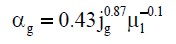 |
| Urseanu et al. [33] | 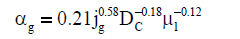 |
| Hikita et al. [29] | 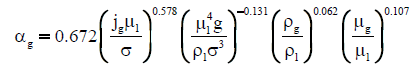 |
| Joshi et al. [7] | 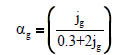 |
| Kawase & Moo-Young [18] | 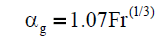 |
| Kawase et al. [36] | 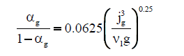 |
| Dimentiev et al. [34] | 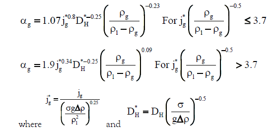 |
| Toshiba et al. [35] | 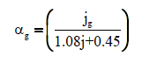 |
Table 1: Gas holdup empirical correlations for bubble column.
For multiple-point measurements, researchers often measure data over a diagonal line with limited radial locations. In contrast, computational power and numerical approaches have become useful tools for predicting those parameters with no interferences. With the rapid advancement of state-of-the-art computational fluid dynamics (CFD) methods, detailed CFD models for the system can be implemented for the design and optimization of the processes while minimizing the need for expensive and time-consuming experimental methods. Using a pilot-scale experiment for CFD validation, a CFD-based scale-up approach could result in more rapid process development at a much lower cost. Consequently, numerous studies have been employed to apply numerical analyses of hydrodynamic behaviours inside bubble column reactors. For instance, Sanyal et al. [43] proposed a two-dimensional axisymmetric model using the commercial CFD software FLUENT and compared the results obtained from the slip mixture model and the two-fluid Eulerian-Eulerian approach with experimental data. This approach is a simplified version of the bubble column, assuming that there is an axial symmetric phenomena that is not quite fitted completely to reality.
A comprehensive study by Joshi reviewed the computational flow modelling efforts to understand the flow patterns in the last three decades [40]. He presented the effects of the superficial gas velocity, column diameter and bubble slip velocity on the flow pattern. Bai et al. studied the impact of the gas sparger on the liquid velocity, void fraction, turbulent kinetic energy and gas-phase mixing of a square bubble column using the Eulerian-Lagrangian approach [16]. One of the main shortcomings of some of these approaches is that their experiments do not cover a wide range of operating conditions. In addition, the results depend on the regime prevailing in bubble columns. In other words, most of them are only valid for a specific regime, either homogeneous or heterogeneous; therefore, the accurate prediction of void fractions and flow patterns over a broad range of operating conditions cannot be guaranteed. In particular, the estimation of the flow pattern in a transition regime needs careful accuracy to obtain reliable results. Because the hydrodynamics of the system at the transition point are thoroughly different from either the homogeneous or heterogeneous regimes, the correlations derived for a specific regime are not valid for the transition pattern. In addition, a majority of previous studies have focused only on continuous bubble column reactors, not semi-batch reactors. However, it is a fact that the pharmaceutical and biotech industries primarily use semi-batch reactors. Many industrially important fermentation and bioreactor operations are carried out in semi-batch mode (e.g., fed batch reactors), producing a wide variety of products [44,45].
Furthermore, semi-batch reactors are used when a reaction has many unwanted side reactions, or when it has a high heat of reaction. By limiting the introduction of reactants, potential problems are eliminated. The main purpose of this work is to present a CFD method to evaluate the parameters of the driftflux model, including the distribution parameter (C0) and drift velocity (C1) over a wide range of flow regimes, from homogeneous to heterogeneous, via the implementation of CFD for a gas-liquid system.
In spite of many variables involved in two-phase flow, the diversity of possible flow patterns makes it more complicated. Therefore, the flow characterization of bubble column reactors affects the performance of the columns significantly. Since the results obtained by experimental or computational investigations depend strictly upon the regime that predominates in the column, identifying the flow structure is of considerable importance. The flow regime in bubble columns is categorized based on superficial gas and liquid velocities, column diameter and fractional gas holdup. Hyndman et al. [46], Kazakis et al. [47] and Shen et al. [41] each classified flow structure in bubble columns into three regimes: the homogeneous (bubbly flow) regime, the heterogeneous (churn-turbulent) regime and slug flow regime. A slug flow regime is only observed at high gas flow rates and in small diameter columns up to 150 mm, producing large cap bubbles (greater than 100 mm) in the column [24,46]. Since the diameter of the bubble column reactor used in this study is 200 mm, this article focuses only on homogeneous and heterogeneous regimes.
The homogeneous regime is observed at low superficial gas velocity (less than 0.05 ms-1 in semi-batch columns) and high superficial liquid velocity. The bubbly flow is characterized by small-dispersed bubbles rising vertically along the main flow direction without any significant dispersion, coalescence or break-up. Consequently, the bubble size distribution is narrow, and the gas holdup profile is uniform in the radial direction. The heterogeneous regime, a socalled churn-turbulent flow, occurs at relatively high superficial gas velocity and is characterized by the existence of a wide range of bubble sizes and vigorous mixing of the liquid phase, which leads to intense local turbulence and secondary flow [17,41,48]. Transition is a change in state wherein one regime is changed to another. Once the transition takes place, the hydrodynamics of the system change dramatically.
Different flow regime maps are proposed in the literature to identify their various conditions. Deckwer et al. presented a flow regime chart for a semi-batch bubble column with a low viscosity liquid phase. According to their map, flow regimes depend on column diameter and superficial gas velocity [49].
Plotting the fractional gas holdup as a function of superficial gas velocity is another approach to identifying different flow patterns. The value of gas holdup increases as the superficial gas velocity increases, but the slope changes during the transition state from one to another. The relationship between α̅g and jg can be correlated by the power law model:

where and jg are overall gas holdup and superficial gas velocity, respectively.
A value of x greater than or equal to 1 indicates the homogeneous regime, whereas x less than one is related to the heterogeneous regime. In the transition regime, the value of x continuously decreases from the higher limit in the homogeneous regime to the lower limit in the heterogeneous regime [17]. However, it is sometimes difficult to distinguish the transition points by using the α̅g-jg graph. To overcome this problem, Wallis proposed the following correlation for drift flux [38].

Where n is a function of the Reynolds number, and  is the
cross-sectional gas holdup [50,51]. For semi-batch reactors, jl is zero,
therefore Eq. (2) can be rewritten as follows:
is the
cross-sectional gas holdup [50,51]. For semi-batch reactors, jl is zero,
therefore Eq. (2) can be rewritten as follows:

Camarasa et al., Shaikh and Al-Dahhan and Kim et al. defined that the value of (n-1) is almost unity for low viscosity liquids [13,22,27]:

They suggested that the plot of  versus αg is an appropriate
graphical method for determining the flow regime. The point at
which the slope of the line changes shows the transition boundary
conditions.
versus αg is an appropriate
graphical method for determining the flow regime. The point at
which the slope of the line changes shows the transition boundary
conditions.
As mentioned in the introduction, drift flux theory, introduced by Zuber and Findlay, is one of the most practical and precise theoretical models for the prediction of gas holdup in two-phase flows [37]. In contrast to a two-fluid model, in which each phase is considered separately and conservation equations including mass, momentum and energy must be solved for each phase, the drift flux model considers the mixture as a whole. Furthermore, the influence of non-uniformity in flow and phase holdup distribution profile, and the local relative motion between phases, are taken into account. This approach reduces the number of numerical equations and the resulting complexity of the problem. In addition, this model is a general one that can be applied to any two-phase flow regime.
The one-dimensional drift flux model is expressed by Eq. (5):
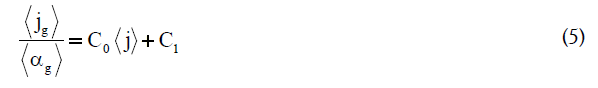
where the < > sign denotes the area average of a quantity over the column cross-section. Distribution parameter (C0) and drift velocity (C1) are defined by Eqs. (6) and (7), respectively.
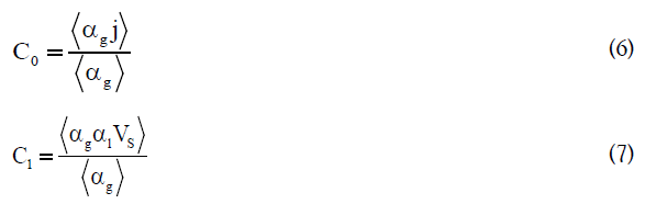
where αg, αl and Vs are the gas void fraction, liquid void fraction and the local relative velocity between phases, respectively. (J=jg+jl) is defined as the mixture’s volumetric flux. C0 represents the intensity of non-uniformity in the void fraction profile, whereas C1 is related to the bubble rise velocity.
According to Eq. (5), when the drift velocity is independent of
fractional phase holdup or, in other words, the flow regime is fully
developed, a plot of jg/αg versus  gives rise to a straight line, in
which the slope of the line represents the distribution parameter
(C0), and drift velocity (C1) can be interpreted by the intercept
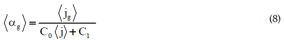
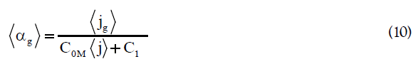
of the graph. The gas holdup equation can be formulated by
rearranging Eq. (5):
gives rise to a straight line, in
which the slope of the line represents the distribution parameter
(C0), and drift velocity (C1) can be interpreted by the intercept
of the graph. The gas holdup equation can be formulated by
rearranging Eq. (5):
By growing development in laboratory instruments and sensors, measuring the local flow parameters C0 and C1 can be obtained based on their definitions. Since the distribution parameter reflects the non-uniformity intensity of the holdup and velocity profile, the C0 close to one indicates the homogeneous regime.
Many studies have been conducted to measure the drift-flux model parameters for various two-phase systems, or to develop empirical correlations in order to reduce the exhausted expensive experimental measurements [37,40,42,52,53].
Despite the simplicity and flexibility of the basic drift flux model,
the model does not take into account the effect of the liquid velocity
profile within the column. As a result, the value of C0 estimated
by Eq. (6) is always different from the value obtained from the
slope of a plot of jg/αg versus . Ranade and Joshi modified the
model proposed by Zuber and Findlay by considering the radial
distribution of liquid velocity. According to their modification, C0 is modified to C0M, and C1 remains the same as Eq. (7) [17].
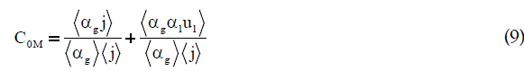
where ul is the local liquid velocity. The second term of the above equation implies the void fraction and velocity distribution due to liquid circulation. As a result, Eq. (8) should be rewritten considering the modification:
Numerous studies have been done to calculate the drift flux model constants and to derive correlations for the distribution parameter and the drift velocity. Some of the proposed equations for the distribution parameter are shown in Table 2.
| Researcher | Distribution parameter |
|---|---|
| Clark & Flemmer [54] | 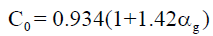 |
| Hibiki & Ishii [55] | 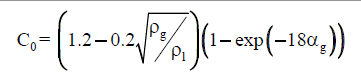 |
| Beattie & Sugawara [56] | 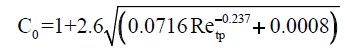 |
| Choi et al. [57] | 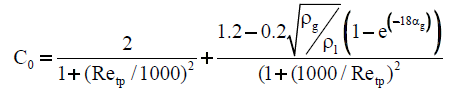 |
| Kataoka & Ishii [34] | 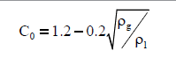 |
Table 2: Correlations for the distribution parameter.
Introduction
Computational fluid dynamics (CFD) is a method for solving conservation equations (partial differential equations) numerically. The conservation equations are: momentum, heat, total mass, and the mass of one species. Considering phenomena in an application, there is almost no analytical solution for all aforementioned equations; hence, we resort to numerical analysis using CFD. This tool equips us to analyze different scenarios that are extremely difficult to obtain through experiments. Empirical correlations and lab- or pilot-scale experiments have shown limitations for chemical engineering process design in terms of cost, scale-up and the optimization of operating conditions. CFD can effectively bridge the gap between large-scale commercialized and lab-scale bubble column reactors and provide a qualitative (and sometimes even quantitative) prediction of velocity, concentration, temperature and pressure profiles.
Various methods with different levels of complexity, ranging from a simple homogeneous flow model to multidimensional models, have been developed. Two forms of CFD models. i.e., Eulerian-Eulerian and Eulerian-Lagrangian approaches are mostly used to simulate the hydrodynamics of two-phase flow in bubble columns. The Eulerian-Eulerian approach represents each phase as an individual interpenetrating continua, where the volume of a phase cannot be occupied by another phase [54-57] while in Eulerian-Lagrangian method the individual bubbles of the gas phase are tracked by writing a force balance for each bubble [2]. The Lagrangian motion of bubbles is coupled with the momentum balance (Eulerian) equation for the liquid phase via the source interaction term and the volume fraction of the gas.
Governing equations
Computational fluid dynamics is based on conservation equations. These partial differential equations (PDE) describe how the velocity, pressure, temperature and density of a moving fluid are related. CFD is the art of replacing such PDE systems with a set of algebraic equations that can be solved using numerical methods. Considering the liquid phase (αl) as continuous and the gas phase (αg) as a dispersed phase, these equations without mass transfer are as follows:
• Continuity equation:
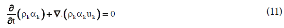
• Momentum equation:
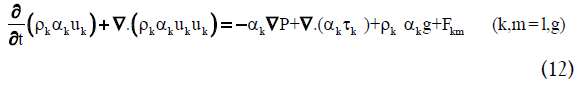
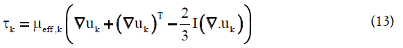
The right hand side of Equation (12) represents all the forces exerted on each phase in every control volume, including pressure gradient, viscous stress, gravitational force and the momentum exchange between phases, respectively. The last term is due to interfacial forces such as drag force FD, lift force FL, virtual mass force FVM and wall lubrication force FWL. Additional closure relations are required to define the viscous stress and interfacial forces. The stress tensor for phase k is described as follows:
The effective viscosity of the liquid phase is composed of the molecular viscosity (μl) and the turbulent viscosity (μT,l).

When the k-ε model is used, the turbulent viscosity is formulated as below:
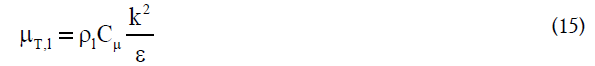
In the above equation, μl is the molecular viscosity of the liquid phase, and Cμ=0.09. The effective viscosity of the gas phase is related to the effective liquid velocity:
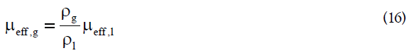
The details of closure models can be found elsewhere [58,59].
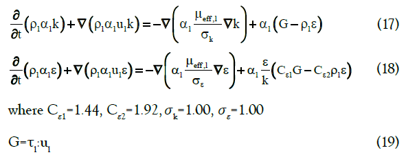
One of the most practical closure correlations for stress tensor, particularly in engineering flow studies, is provided by the standard k-ε model. It describes the turbulence characteristics by means of two transport equations. The first equation determines the energy in the turbulence of so-called turbulent kinetic energy (k). The second transport equation implies the rate of dissipation of the turbulent kinetic energy (ε). These two definitions are given in the following transport equations:
To obtain a reliable model to simulate a multiphase flow, the precise selection of closures for interfacial forces is vital. Taking into account all forces leads to a complicated model that is not only computationally expensive but can also cause convergence problems for solving systems of equations using iterative methods. Therefore, choosing the interactions between phases is of considerable importance. The interfacial forces involved in momentum equations are mainly caused due to the transfer of momentum from one phase to another, and many efforts have been made to study the effect of interfacial forces on flow patterns in bubble column reactors [10,60-63]. In general, in two-phase flows with constant slip velocity, drag force prevails over other possible forces. Laborde-Boutet et al. [64] used custom-field functions to compute the magnitude of different interaction forces. They confirmed that the intensity of drag force is 100 times greater than other forces. Drag is a force that acts opposite to the relative motion of bubbles moving with respect to the surrounding fluid. The drag force is expressed by the following:
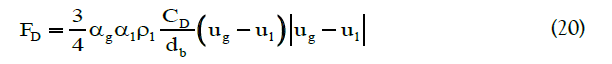
where CD is the drag coefficient. In the present work, we used the drag coefficient proposed by Schiller and Naumann:
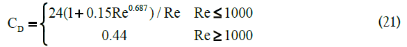
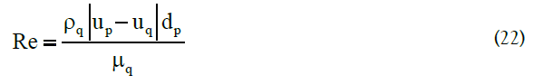
Re is the relative Reynolds number. The relative Reynolds number for the primary phase of q and the secondary phase of p is calculated as the following equation:
In the case of non-uniform motions, rising bubbles experience some lateral forces in the radial direction, such as virtual mass force and lift force. Joshi [40] and Simmonet et al. [61] found that, without considering virtual mass force, calculations lead to divergence and cannot predict a realistic gas holdup profile and transient characteristics. A constant virtual mass coefficient of 0.5 was assumed. It is worth noting that although many studies have been conducted on the lift force [65-67], there is a dispute regarding the magnitude and the sign of the lift force and it has not yet been properly modeled for the inclusion in Eulerian-Eulerian method [68,69]. In addition, according to our observations, applying lift force results in extreme convergence problems and unstable calculations, while by neglecting this secondary force, the model still predicts the experimental data very well. Because of these uncertainties and based on the several published studies on bubble column that shows this force is either negligible compared to the drag force or not yet properly modeled [64,68-71], only drag force and virtual mass force are taken into account for the current simulation.
In addition to taking account the interfacial forces and the turbulence model, the appropriate selection of bubble diameter plays an important role to achieve an accurate model so that can be able to predict the actual flow behaviour. Although some of the studies have used the population balance models to simulate the evolution of bubble size, however, the complexity of these models introduces additional uncertainties [72]. Moreover, some other researchers showed that implementation of bubble population balance models, yields to a significant underestimation of bubble break-up rates and turbulence stress [69,70,73,74]. In this respect, it is reasonable to use the single bubble size that has been also applied in most of the previous works.
Simulation details
This study tried to simulate the experimental setup used by Sasaki et al. [75]. The three dimensional geometry of a cylindrical air-water bubble column reactor with a diameter of 200 mm and total height of 2000 mm was generated by means of the commercial CFD code ANSYS® FLUENT 16.2. The mesh independency study was carried out using 28665, 60032 and 119168 numbers of elements. The gas holdup and gas velocity profiles were monitored for all numbers of meshes. It was observed that the results for cases 60032 and 119168 are almost the same; therefore, since the coarser grid is computationally less expensive but still provides a sufficient level of accuracy, the mesh with 60032 elements was selected for the rest of the simulation. A mono-dispersed bubble size distribution with a mean bubble size of 5 mm was considered. The column was initially filled with water to a height of 1000 mm as the continuous phase. The bottom of the column was specified as an inlet, and air was introduced to the column inlet, as the dispersed phase, with superficial gas velocity ranging from 0.025 to 0.4 ms-1. Outflow and no-slip boundary conditions were applied to the outlet and the walls of the column, respectively. An Eulerian-Eulerian model was solved using the pressure-based solver. The phase-coupled SIMPLE algorithm, which is a modification of the SIMPLE scheme, was selected as the pressure-velocity coupling method. The governing equations were spatially discretized using the Green- Gauss Cell-Based approach, and QUICK and modified HRIC were used as discretization methods for momentum and volume fraction, respectively. A transient model with a time step of 0.01 s was considered, and the number of iterations per time step was 50, to ensure that every time step met the convergence criteria. Simulations were performed until a quasi-steady state was reached. During this stage of simulation, the level of the interface was monitored. An indication of the quasi-steady state is a dynamically stabilized interface. We also monitored the area-average void fraction for gas at some representative points in the column, as indications of flow development until it leveled off to a constant value. Generally it takes about 40 s for the simulation to reach the quasi-steady state. The model was simulated for 100 s, while data were time-averaged at steady state conditions over the last 60 s.
Gas holdup and flow structure
As previously mentioned, gas holdup plays a significant role in
the design and scale-up of bubble column reactors. Figure 1 shows
the effect of superficial gas velocity on the overall gas holdup,
calculated by a computational model (this work), compared
with the experimental results presented by Sasaki et al. [75]. The
predicted overall gas holdup values are in good agreement with the
experimental results. The fractional gas holdup increases as inlet
gas velocity increases. However, a sharper slope is observed for
jg<0.05 ms-1 and gradually decreases by increasing the gas velocity.
For velocities less than 0.05 ms-1, jg is proportional to so that,
according to criteria discussed in Flow Patterns section, it indicates
a homogenous regime, whereas jg is proportional to
so that,
according to criteria discussed in Flow Patterns section, it indicates
a homogenous regime, whereas jg is proportional to  − for jg>0.2
ms-1, implying a heterogeneous regime. The slope change can be
explained by the transition from bubbly to cap-bubbly flow. The
transition occurs when too many small bubbles exist as a result
the bubbles cannot move between each other without collision,
which results into the coalescence of the bubbles into larger stable
bubbles. Transition regime occurs in gas velocities varying from
0.05 ms-1 to 0.2 ms-1. It can be concluded that the α̅g - jg relationship
depends upon the flow pattern of operations.
− for jg>0.2
ms-1, implying a heterogeneous regime. The slope change can be
explained by the transition from bubbly to cap-bubbly flow. The
transition occurs when too many small bubbles exist as a result
the bubbles cannot move between each other without collision,
which results into the coalescence of the bubbles into larger stable
bubbles. Transition regime occurs in gas velocities varying from
0.05 ms-1 to 0.2 ms-1. It can be concluded that the α̅g - jg relationship
depends upon the flow pattern of operations.

Figure 1: Overall gas holdup at different superficial gas velocity.
Since the α̅g - jg graph does not have a maximum, it is somewhat difficult to specify the transition point. In order to determine the flow regimes more precisely, Sasaki et al. [75] suggested a plot of the gradient dα̅g/djg versus jg, which is illustrated in Figure 2. It can be observed that the slope of the plot decreases with increasing superficial gas velocity for jg<0.2 ms-1 and it levels off to an almost constant value for jg>0.2 ms-1. Consequently, this plot verifies the different flow patterns obtained by Figure 1.

Figure 2: Estimating of flow regimes with Gradient dα̅g /djg.
The other method for determining the flow regime is based on
the drift flux theory. A plot of  versus
  , shown in Figure 3, was used for a better description of flow patterns. Regime
transition can be easily recognized by changing the slope of the
graph. Analyzing this figure reveals that gas holdup larger than 0.25
reflects a heterogeneous regime, and gas holdup less than 0.08 is
related to a homogeneous regime. In this method, cross-sectional
gas holdup is used instead of overall gas holdup.
, shown in Figure 3, was used for a better description of flow patterns. Regime
transition can be easily recognized by changing the slope of the
graph. Analyzing this figure reveals that gas holdup larger than 0.25
reflects a heterogeneous regime, and gas holdup less than 0.08 is
related to a homogeneous regime. In this method, cross-sectional
gas holdup is used instead of overall gas holdup.
| Researcher(s) | Fluid system | Column diameter [m] | Superficial gas velocity [ms-1] | Pressure [MPa] | Viscosity [Pa.s] |
|---|---|---|---|---|---|
| Hills [66] | Air- Water | 0.15 | 0.04-0.4 | 0.1 | 0.001 |
| Urseanu [33] | N2-Water | 0.15 | 0-0.40 | 0.1, 0.5 | 0.001 |
| N2-Tellus oil | 0.15 | 0-0.25 | 0.1, 0.8 | 0.07 | |
| N2-Glucose A | 0.15 | 0-0.25 | 0.1-1.0 | 0.17 | |
| N2-Glucose B | 0.15 | 0-0.15 | 0.1-1.0 | 0.55 | |
| Schlegel et al. [72] | Air-Water | 0.152 | 0-0.50 | 0.1 | 0.001 |
| Esmaeili [73] | Air-Water | 0.292 | 0-0.25 | 0.1 | 0.001 |
| Gemello et al. [74] | Air-Water | 0.40 | 0.03-0.35 | 0.1 | 0.001 |
Table 3: Databases used in this study.

Figure 3: Estimating of flow regimes with drift flux mode.
Radial distribution of time-averaged gas holdup computed at different heights of the Column (height to diameter ratio; z/ D=0.75-5.0) and various superficial gas velocities (jg=0.025-0.4 ms-1) are illustrated in Figure 4. The figure shows that the radial gas holdup changes from a wall-peaked shape at the bottom of the column to a center-peaked profile at higher levels. At the lower levels bubble diameter is smaller than at the higher levels because as the level increases the bubble size increases as a result of coalescence/ dispersion. The balance between the coalescence and breakage as well as the reduced static pressure at higher axial positions lead to create larger bubbles which tend to migrate toward the center of the column. Furthermore, the gas holdup profile is radially uniform at low gas velocities, implying a homogeneous regime, but it is almost parabolic at higher velocities, corresponding to transition and heterogeneous regimes.

Figure 4: Radial distribution of gas holdup at various superficial gas velocities.
Distribution parameter
As discussed in Drift Flux Theory section, since the non-uniformity
in velocity and gas holdup is taken into account in the definition
of the distribution parameter and drift velocity, flow patterns
can be directly concluded by analyzing these two parameters.
Based on a one-dimensional drift flux model, Eq. (5), C0 and C1 are obtained by the slope and intercept of  versus
  in
a fully developed flow. However, the majority of two-phase flows
in large diameter columns are not fully developed; as a result, the
parameters obtained by graphical methods may not predict the real
flow behaviour. By using CFD and computing local velocity and
void fraction profiles, it is possible to calculate the distribution
parameter and drift velocity by their definitions according to Eqs.
(6) and (7), respectively. The modified distribution parameter (C0M)
is defined by Eq. (9), considering the influence of liquid circulation. Figures 5 and 6 show the effect of a wide range of superficial gas
velocities, covering different flow regimes, on C0 and C0M. Both
graphs show a similar trend; however, the value of C0 estimated
by Eq. (6) is lower than the C0M values obtained by Eq. (9), which
is caused by considering the effect of liquid circulation in the
definition. It can obviously be seen that the distribution parameter
is not a constant value with respect to superficial gas velocity. This
may explain the reason for the different values of the distribution
parameter reported in the literature. According to Figure 6, C0M is
almost unity at low velocities (jg<0.05 ms-1), dramatically increases
to a maximum at 0.1 ms-1 and then decreases to a value of 1.5. This
behaviour clearly verifies the description of regimes. C0M equal to
1 implies a uniform gas holdup profile and, as a result, represents
the homogeneous regime. By further increasing in the gas velocity,
internal circulation starts and leads to an intense non-uniformity
in the radial holdup distribution, so that the transition regime
occurs. This process results in a sharp increase in the distribution
parameter up to the beginning of the heterogeneous regime. In
the heterogeneous regime, as gas velocity increases, the turbulent
also intensity increases and tends to reduce the non-uniformities.
Therefore, the amount of C0M decreases gradually.
in
a fully developed flow. However, the majority of two-phase flows
in large diameter columns are not fully developed; as a result, the
parameters obtained by graphical methods may not predict the real
flow behaviour. By using CFD and computing local velocity and
void fraction profiles, it is possible to calculate the distribution
parameter and drift velocity by their definitions according to Eqs.
(6) and (7), respectively. The modified distribution parameter (C0M)
is defined by Eq. (9), considering the influence of liquid circulation. Figures 5 and 6 show the effect of a wide range of superficial gas
velocities, covering different flow regimes, on C0 and C0M. Both
graphs show a similar trend; however, the value of C0 estimated
by Eq. (6) is lower than the C0M values obtained by Eq. (9), which
is caused by considering the effect of liquid circulation in the
definition. It can obviously be seen that the distribution parameter
is not a constant value with respect to superficial gas velocity. This
may explain the reason for the different values of the distribution
parameter reported in the literature. According to Figure 6, C0M is
almost unity at low velocities (jg<0.05 ms-1), dramatically increases
to a maximum at 0.1 ms-1 and then decreases to a value of 1.5. This
behaviour clearly verifies the description of regimes. C0M equal to
1 implies a uniform gas holdup profile and, as a result, represents
the homogeneous regime. By further increasing in the gas velocity,
internal circulation starts and leads to an intense non-uniformity
in the radial holdup distribution, so that the transition regime
occurs. This process results in a sharp increase in the distribution
parameter up to the beginning of the heterogeneous regime. In
the heterogeneous regime, as gas velocity increases, the turbulent
also intensity increases and tends to reduce the non-uniformities.
Therefore, the amount of C0M decreases gradually.

Figure 5: The effect of jg on the distribution parameter.

Figure 6: The effect of jg on the modified distribution parameter.
Figure 7 renders a comparison between the values of C0 and C0M computed using the CFD model, the experimental data and some of the empirical correlations presented in Table 2. The experimental data by Dharwadkar [17], which covers a wide range of jg were used to investigate the effect of superficial gas velocity on the distribution parameter.

Figure 7: Comparison of the distribution parameter calculated by different models.
A closer look into the plot indicates that the values of C0M, computed by means of the proposed CFD model in this study, agree reasonably well with the experimental data by Dharwadkar, whereas the empirical correlations are in fairly good agreement with the values of C0. This deviation can be justified by recalling that many researchers have not taken the effect of liquid circulation into consideration. By contrast, all of the existing constitutive equations for the distribution parameter have been derived for a continuous bubble column (i.e., in the presence of net liquid flow) [76-79].
Drift velocity
The values of C1 were calculated based on Eq. (7), and results are illustrated in Figure 8. It can be concluded from this graph that, by enhancing superficial gas velocity, the drift velocity increases. This can be explained by the fact that the size of bubbles increases with the enhancement in jg. These larger bubbles rise faster in the axial direction, resulting in an increase in the overall bubble rise velocity. In addition, the pressure decreases in the direction of the bubbles’ movement. The generated drag force acts opposite to the relative motion of the bubbles, with respect to the surrounding fluid, which leads to a decrease in drag coefficient and an increase in the slip velocity. The same effect reduces the slip velocity near the wall, where there is a downward flow. However, since the number of bubbles is greater in the centre of the column, the overall slip velocity and consequent drift velocity are higher at higher superficial gas velocities. The values of C1, obtained by CFD were verified by the experimental data of Dharwadkar [17].

Figure 8:The effect of jg on the drift velocity.
Both C0M and C1 values calculated by the CFD model are higher than the experimental results. However, since Dharwadkar did not mention any uncertainty regarding their measurements (the error bars) in their paper and emphasized the fact that CFD models are an averaging of many steps in transient studies, this inconsistency might be justified for this study. In addition, the used models have their own limitations (especially the Eulerian-Eulerian model). Overall, the computationally calculated drift-flux parameters are in good agreement with the experimental results and can be used as a reliable method for estimating the gas holdup in bubble column reactors. In order to show the reliability of the present model for the prediction of gas holdup, the results from the simulation are plotted against the gas holdup equations obtained from Table 1 and the values directly obtained by using the drift-flux model, as shown in Figure 9. The comparison of the numerical and experimental results leads to a good match, except for the correlation proposed by Dimentiev [34].

Figure 9:Gas holdup prediction by using different models.
On basis of the results obtained in this study, following equation can be proposed, to predict the fractional gas holdup for semi-batch bubble column reactors as a function of superficial gas velocity. To validate the reliability of the presented model, it was compared with CFD results and the experimental data available in literature, as shown in Figure 10. The dataset used in this study are listed in Table 3. The proposed correlation predicts the gas holdup very well compared to the experimental data with an R2 equal to 0.973.
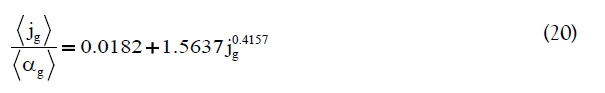

Figure 10:Comparison of the proposed model against the experimental data.
In view of the wide application of bubble column reactors and the necessity of developing a flow pattern-independent model to design and scale-up these operation units, a numerical simulation over a wide range of superficial gas velocity was conducted via implementation of ANSYS® FLUENT 16.2. However, because of the importance of the drift-flux model as a practical method for predicting the fractional gas holdup, the distribution parameter and the drift velocity were determined directly by their definitions. To yield a more precise prediction of the real system, the effect of liquid circulation was taken into account. The results can be summarized as follows:
• The overall gas holdup increases as the superficial gas velocity increases. The predicted overall gas holdup values are in good agreement with the experimental results.
• Two methods were performed to determine the flow structure,
and three regimes were distinguished, namely, homogeneous
(bubbly flow), transition and heterogeneous (churn-turbulent flow).
The plot of  versus jg shows the homogeneous regime for
jg<0.05 ms-1and the heterogeneous regime for jg>0.2 ms-1, whereas
the plot of
versus jg shows the homogeneous regime for
jg<0.05 ms-1and the heterogeneous regime for jg>0.2 ms-1, whereas
the plot of  versus categorizes the flow structure
based on cross-sectional gas holdup. For this study, <0.08
was identified as the bubbly flow, while churn-turbulent flow was
observed for >0.25.
versus categorizes the flow structure
based on cross-sectional gas holdup. For this study, <0.08
was identified as the bubbly flow, while churn-turbulent flow was
observed for >0.25.
• The distribution parameter C0M represents the uniformity of the radial holdup profile, which depends upon the movement of bubbles in a radial direction. C0M closer to unity indicates the uniform profile and, as a result, the homogeneous regime. In contrast to the basic drift-flux theory, C0M is not a constant value and varies via changes in superficial gas velocity. It is almost unity at low velocities ( jg≤ 0.05 ms-1), dramatically increases to a maximum at 0.1 ms-1 and then decreases to a value of 1.5.
• The drift velocity C1 implies the bubble rise velocity. This parameter also differs at different superficial gas velocities. The value of C1 increases by raising the superficial gas velocity.
• The existing constitutive correlations for the distribution parameter cannot predict the hydrodynamics of semi-batch bubble columns.
A flow pattern-independent correlation, as a function of superficial gas velocity, was proposed to predict the gas holdup without any need for experimental data.
Citation: Bahramian A, Elyasi S (2019) A Numerical Model for Bubble Column Reactors: Prediction of the Fractional Gas Holdup by the Implementation of the Drift-Flux Model. 9: 396. DOI: 10.35248/2157-7048.19.10.396
Received: 27-Jun-2019 Accepted: 29-Jul-2019 Published: 05-Aug-2019 , DOI: 10.35248/2157-7048.19.10.396
Copyright: © 2019 Bahramian A, et al. This is an open-access article distributed under the terms of the Creative Commons Attribution License, which permits unrestricted use, distribution, and reproduction in any medium, provided the original author and source are credited.