Advancements in Genetic Engineering
Open Access
ISSN: 2169-0111
ISSN: 2169-0111
Research Article - (2016) Volume 0, Issue 0
This paper mainly concentrates on image segmentation using Wavelet, otsu and Curvelet algorithm. The existing Chan Vese model becomes complex in determining multiple images simultaneously in varying intensities. In order to increase the detection performance the WOC (wavelet Otsu curvelet) algorithm is proposed. Due to high directionality and anisotropic nature of the curvelet transform, it gives better performance at the edges and it is also applied for multi-scale edge enhancement. Wavelet transform is well suited for multi resolution. Wavelet and curvelet transforms are incorporated for sub band decomposition of frequency coefficients. Otsu algorithm has a novel approach for segmentation where thresholding is done using histogram analysis. This in turn reduces the segmentation complexity and hence the new algorithm is termed as Hybrid fast WOC algorithm.
<Keywords: Wavelet; Curvelet; Ridgelet; Histogram; OTSU; Segmentation
Image segmentation is the division of an image into different regions, each possessing specific properties. Once the image has been segmented, measurements can be performed on each region and the characteristics features between adjacent regions can be investigated. Image segmentation is therefore a key step towards the quantitative interpretation of image data. Some of the practical applications are medical imaging, biomedicine, object recognition; detection etc. Initially pre-processing is done to de-noise the image for further segmentation. The low level processing methods transforms the image to high level image description in terms of features and objects.
The shapes of cells are evolved by the influence of Chan-Vese model tracking method which detects multiple cells simultaneously by diffusion filtering and boundary detection. The 2D and 3D time lapse series gets complicated with tightly packed high density cells [1]. Magnetic Resonance Imaging (MRI) used to improve the quality of an image by de-noising and resolution enhancement before preprocessing an image for any application. The mean, median, wiener filtering and discrete wavelet transform (DWT) are used for de-noising and enhancement purpose for any image [2].
The ultrasound images contain speckle noise, creating a circular granular pattern Balzaachmad et al., [3] which degrades the quality. Thus wrapping and de-wrapping operations are done prior and after the application of anisotropic diffusion. Wiener filtering technique minimizes the mean squared error initially before high level processing [4]. This method is fast by requiring only the computation of the certainty map and a sequence of linear filtering, which outperforms the nonlinear methods like anisotropic and diffusion filtering. Segmentation by watershed distance transforms [5] is complex due to multiple partitioning and overlapping of objects.
The wavelet transform Gavlasova et al., [6] is used for feature extraction in multi-dimensional signal processing. Wavelet frames are applied in image restoration problems, such as de-noising, de-blurring, etc. A convex multi-phase segmentation model Tai et al., [7] is used that allows to automatically identifying the complex tubular structures, including blood vessels, leaf vein system, etc. Incorporating the low frequencies of the frame let transform of an image has additional advantages, such as to speed up the convergence of the algorithm and yield a binary solution. Multi-resolution analysis (MRA) Kulkarni et al., [8] allows the preservation of an image according to the levels of blurring. It aims at automatic image separation for classifying the region where each layer is split into a number of layers and wavelet transform is used for image extraction. For resolution enhancement, SWT (Stationary Wavelet Transform) Prasad et al., [9] decomposes the image into sub bands. The high frequency coefficients have been multiplied with the orthogonal matrix coefficients. The low resolution input image and high frequency sub band images are interpolated using bi cubic interpolation. Inverse integer wavelet transform has been used to combine all these sub images for a better equalized image.
The ridgelet transform applies to complete wavelet pyramid whose wavelets has compact support in the frequency domain. The curvelet transform [10] is non-orthogonal having curvelet sub bands using a filter bank. The implementation of both the curvelet and ridgelet transform results in exact reconstruction property. Thus it de-noises some of the standard images. Moreover, the curvelet reconstructions exhibit higher perceptual quality than wavelet-based reconstructions, offering visually sharper images with higher quality, recovery of edges and curvilinear features. The potential applicability of ridgelet and curvelet transforms has multi-scale analysis and geometry ideas answering to a wide range of image processing problems. The decomposition is based on the coefficients of curvelet transform segmented by N-cut algorithm Al-Saif et al., [11] then the segmented edge will be inserted in the original image to make separation between different segments [12].
The digital image of retina is segmented with contrast adjustment using multi scale method to increase the dynamic range of gray levels. The morphological operators are used to smoothen the background allowing vessels to be seen clearly by eliminating the non-vessel pixels [13]. The texture analysis characterizes tissues to determine changes in the functional characteristics of organs at the onset of disease. This approach has two steps namely the extraction of the most discriminative texture region and creation of classifier for identification [14]. Curvelet transform deals with interesting phenomena occurring along the curves. It reveals optimal representation of the region of interest (ROI) with better accuracy, less noise and shows good renewal of the edge data by integrating a directional component [15]. Ridgelet gives rise to a framework for constructing a number of other affine invariant transforms that offers the possibilities for variation. It illustrates that ridgelet invariants extract highly discriminative and robust information from image patches [16].
The target image is acquired by separating the target from background image for morphology analysis. Then, the mono layer wavelet coefficient is applied to separate the target image and redundant information is removed by means of low frequencyreconstruction. Otsu algorithm is used to detect the surface defects [17]. The diffusion preprocessing is followed by exploiting the link of a new hybrid numerical technique for segmentation. Otsu is an automatic threshold selection [18,19] of an optimal gray-level threshold value for separating objects of interest in an image based on their gray-level distribution.
To obtain better segmentation results with reduced complexity when compared to previous algorithm, WOC (wavelet Otsu curvelet) method is incorporated and it is prescribed in the following flow diagram Figure 1.

Figure 1: Flow diagram of segmentation
Anisotropic diffusion
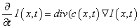
Anisotropic diffusion removes noise without blurring the edges in digital images. It is mathematically formulated as a diffusion process that encourages smoothing within a region in respect to smoothing across the boundaries. In this filtering method the estimation about local image structure is guided by knowledge about the statistics of the noise degradation and the edge strengths. The anisotropic diffusion is described as [2,3] in the equation 1.
 (1)
(1)
Where denotes the gradient, div function denotes the divergence operator and c(x,y,t) is the diffusion coefficient. The (x,y) represents spatial coordinates and t is used for enumerating iteration steps. I represent the intensity function of an image. c(x,y,t) regulates the rate of diffusion by preserving the edge details in an image by considering the gradient parameter. This function c(x,y,t) is a non-negative monotonically decreasing function. This function diffuses within regions and does not affect region boundaries that are at locations of high gradients. The function for the diffusion coefficient is described in equation (2).
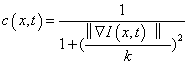 (2)
(2)
The constant K is experimentally chosen which manipulates the sensitivity of edges and acts as a function of noise.
Wiener filter
The fundamental problem of ultrasound images is the poor quality mainly caused by multiplicative speckle noise. Speckle noise is a random mottling of the image with bright and dark spots which reduces [4] fine details and degrades the detectability of low contrast region. Occurrence of speckle noise is adverse since it alters the tasks of human elucidation and diagnosis. In order to remove this speckle noise one efficient method is to go for wiener filter.
A Wiener filter is a minimum mean square error filter. It has capabilities of handling both the degradation function as well as the noise unlike the inverse filter. It is adopted for filtering in the spectral domain. By applying inverse filtering original image is recovered. This filtering technique is sensitive to Gaussian noise, Hence wiener filter is used to remove noise from image by inverting the blurring effect simultaneously. Thus the wiener Filter reduces the mean square error by the smoothing process. And it gives a linear estimate of an input image. In Fourier domain wiener filter function is prescribed in equation 3.
F(u,v)=[H(u,v)/|H(u,v)|2+Sη(u,v)/Sf(u,v)]G(u,v) (3)
Where F(u,v) is estimate of undegraded image. H(u,v) is the degradation function. H(u,v) is the complex conjugate of H(u,v). | H(u,v)2|=H(u,v)H(u,v)Sη(u,v)=|N(u,v)| 2 is the power spectrum of the noise. Sf(u,v)=|F(u,v)| 2 is the power spectral density (PSD) of the un degraded image and G(u,v) represents degraded image.
The above expression is based on the following assumptions:
1. The noise and the image are uncorrelated
2. The noise or the image has zero mean
3. The gray levels in the estimate are a linear function of the levels in the degraded image. The Wiener filter handles the situation in which the degradation function is zero, unless both the degradation function as well as the noise power spectrum is zero.
Top and bottom hat approach
The luminous area and dark area are eliminated by the performance of morphological top hat and bottom hat filtering an input image before segmentation. The enhanced version of image is obtained by taking the difference between the top hat and bottom hat filtered images. Thresholding is carried out in wavelet transform to segment the enhanced image from different regions and then finally fuse them by performing inverse wavelet transform. The top-hat transformation of a gray scale image T(f) is defines as the equation 4.
T(f)=f–(fb) (4) Similarly, the bottom-hat transformation of a gray scale image f is defines as the equation 5.
B(f)=f.b–f (5)
One principal application of these transforms is in removing objects from an image by using structural elements in the opening and closing that does not fit the objects to be removed. The difference then yields an image with only the removed objects. The top-hat is used for light objects on a dark background and the bottom-hat-for dark objects on a light background.
Curvelet transform is a special member of the emerging family of multi scale geometric transforms, it was developed in the last few years as an attempt to overcome inherent limitations of traditional multi scale representations such as wavelet transform and Fourier transform. In existing Fourier transform, the co-efficient are affected by point discontinuities and so wavelet transform is implemented to prevent these point discontinuities. But the wavelet co-efficient are affected by curve discontinuities which can be minimised by using curvelet transform and gives better directionality to edges. This curvelet transform detects the curves with very less co-efficient when compared with wavelet transform. The application of this first generation curvelet transform is very much limited excluding the blocking effect. These limitations are mainly due to the geometry of ridgelet as they are not sure of ridge functions in digital images [10] Successively, a simpler second-generation curvelet transform was evolved which is based on frequency partition technique. This second-generation curvelet is proved as an efficient tool for various applications in digital image processing. The following steps indicated below exhibits the overview of curvelet transform [12] Figure 2.

Figure 2: Steps involved in the Curvelet transform
Subband decomposition
Sub-band decomposition Fadili [12] techniques have been extensively used for data coding and analysis. The decomposition of the original signal into different sub images is called sub band decomposition. The decomposition process is recursively applied to the low-frequency sub-band to generate the next level of the hierarchy. The scaling filters are applied in both the horizontal and vertical directions followed by a 2-1 sub-sampling of each output image. This generates three orientation selective detail images Dj, k and a coarse or approximate image Cj, where k=1,2,3 and j represents the level of decomposition. The next level of decomposition is produced by repeating the same process. The decomposition of an image is implemented with wavelet decomposition
Wavelet decomposition: Image de-noising is the pre-processing method which involves the influence of the image information to yield a visually high quality image. There are many methods for removing noise from an image like wavelet decomposition. It is a technique that decomposes an input image into different sub images to get the wavelet co-efficient [20]. These co-efficient are then de-noised with a particular wavelet threshold. Finally the inverse operation is applied to the coefficient in order to obtain the de-noised image.
Wavelet decomposition decomposes an image into different subbands namely LL: obtained by low pass filtering the rows and columns. LH: obtained by low pass filtering the rows and high pass filtering the columns. HL: obtained by high pass filtering the rows and low pass filtering the columns. HH: obtained by high pass filtering the rows and high pass filtering the columns.
LH-low high band which gives vertical information
HL-high low band which gives horizontal information
HH-high high band which gives diagonal information
LL-low low band that consists of low frequency components (i.e.) important information.
The input image is read in form of matrix and is decomposed into n levels producing 2n different set of co-efficient. For a 2D image in a grey scale value is stored in an array which undergoes symmetric periodic extensions along rows and then filtered by low pass and high pass filters along each rows of the array. After filtering along each of the rows it is down sampled by a factor 2 which means every odd sample is eliminated from the array obtained after convolution (multiplication). The same filtering and convolution processes are repeated on columns. Lastly, the resultant array are down sampled by the same factor 2 and thus four sub bands are obtained after the first stage of decomposition Figure 3.

Figure 3: Wavelet decomposition.
Thresholding: Thus the obtained co-efficient are de-noised by fixing a particular threshold. It filters each co-efficient from the sub bands with a threshold function to obtain modified co-efficients. The subbands HHk, HLk, LHk, where k=1,2,3..j are called the details where ’k’ is the scale and ’j’ denotes the largest or coarsest scale in decomposition. The LLk is the minimum resolution pixel.
To remove the unwanted coefficients like noise, threholding is applied to the sub-bands. There are two types of thresholding namely hard and soft thresholding. This thresholding method removes noise while keeping the low resolution co-efficients (important information) unaltered.
In soft threholding, the comparison is made between the detail coefficients and the given threshold [20].These co-efficients are shrinked close to zero to remove the noise in data. Whereas in hard thresholding, the co-efficient is compared with the threshold and is made to zero if the value is less than threshold, else it is remains unchanged based on the threshold rule. Thresholding helps to identify the co-efficients that carry noise and the ones that consist of data signal. Choosing the optimum threshold value is highly important. A small threshold value will restore the noisy co-efficients and high threshold value leads to the loss of co-efficients that carry image pixels. The inverse wavelet transform or reconstruction is done exactly the opposite way to that of the decomposition. Of the four obtained subband images the up sampling is done first followed by filtering applied to the columns and then to the rows to get the reconstructed image.
Smooth partitioning
Partition of the image is used to analyze the curve singularities. So before ridgelet transform partition of the image is made to obtain subimages. The frequency partition is provided to overcome unclear geometry of ridgelet [12] Consider w to be the smooth windowing function with a size of 2 × 2 matrix. This window matrix is multiplied with the function Q and this windowing function wQ produces results localized near Q (∀Q∈Qs). Smooth partitioning of the function into ‘squares’ are represented as equation 6.
 (6)
(6)
Where,
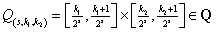 (7)
(7)
Where WQ is window function and Δsf is band of frequency
Re-normalization
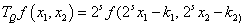
Re-normalization involves centering each dyadic square to unit square [0.1] ×[0.1]. For each Q, [11] the operator TQ is defined as equation 8.
 (8)
(8)
Where k1, k2 are integer values TQ is rescaling operator
The above equation denotes the operator which transports and renormalizes the function f, where the part of the input supported near Q becomes the part of the output supported near [0.1] × [0.1]. In this stage of the procedure, each ‘square’ resulting in the previous stage is re-normalized to unit scale [12].
 (9)
(9)
Where
gQ re-normalized image
Ridgelet analysis
The optimal ridgelet transform involves finding the lines of the size of the image before line segment portioning is introduced. Consider Q as dyadic square and Qs denotes the collection of all dyadic square with the scale of S in which Q € Qs. [16] and with the window w the collection of all dyadic square is denoted as WQ. The ridgelet elements are localized near the square Q. After smooth partioning ridgelet transform is applied to each square. Ridgelet is very efficient in line singularities whereas wavelet is effective only n point singularities. An isotrophic wavelet transform is named as ridgelet transform.
The ridgelet transform is expressed as equation 10.
Rf(a,b,ϴ)=∫ᴪa,b,ϴ(x)f(x)dx (10)
Where
ᴪ a,b,ϴ (x) – Ridgelet function, expressed as
ᴪ a,b,ϴ (x)=a ᴪ((x1 cos ϴ)+(x2 sin ϴ-b)/a). This function is constant along the line. The ridgelet transform satisfy the personal relation. Ridgelet does not provide the right tool for curve singularities. So to achieve this ridgelet further construct a system called curvelet. Curvelet is build with special frequency localization of ridgelet. The ridgelet theory related with Radon transform.
Otsu method helps in automatic thresholding. Image thresholding may be considered as a classification task where a considerable amount of object/class information is embedded in spatial arrangements of intensity values forming different object regions in an image [17]. Thresholding is the key process for image segmentation. Thresholding can be of two types- Bi-level and Multi-level. In Bi-level thresholding, two values are assigned-one below the threshold level and the other above it. In Multilevel thresholding, different values are assigned between different ranges of threshold levels.
Image thresholding is a method which extracts objects in an image from the background. It is one of the most common operations in image processing and such, it has been extensively researched by computer vision experts. Thresholding methods are categorized according to the information they obtain from the data: • Histogramshaped- based • Clustering-based • Entropy-based Attribute similarity methods • Object attribute-based • Spatial approaches • Local methods
Otsu method based on 2D histogram
The objective of thresholding is to extract objects or regions of interest in an image from the background based on its gray level distribution. The histogram approach not only utilizes the gray level distribution of pixels, but also the average gray level distribution of their neighborhood to select the optimal threshold vector. As a step to more in-depth with thresholding analysis, the histograms of the image set were extracted. Image histograms are a useful tool to help discover some properties from images, and even directly obtain thresholds from them. For example, given a simple image with a light object over a dark background, its histogram would be confirmed by two predominant peaks (i.e. a bimodal histogram), so one thresholding value would be enough to correctly segment the image. A morphological analysis of histograms can help predict which thresholding method may offer the best performance for a particular image by reasoning about some assumptions of the thresholding method itself. However, morphological analysis alone is often not sufficient for discovering useful properties in a gray-level image. Histograms are a statistical concept, it makes sense to refer to the average, variance, skewness, entropy and kurtosis of them.
The mean of a data set, and in particular of an image histogram, is the arithmetic average of the values in the set, obtained by summing all values and dividing by the number of them. The mean is, thus, a measure of the center of the distribution. The mean is a weighted average where the weight factors are the relative frequencies. It was calculated for the histograms of this experiment because it provides information about the brightness level of an image. The variance of a data set is the arithmetic average of the squared differences between the values and the mean. The standard deviation is the squared root of the variance. The variance and the standard deviation are both measures of the spread of the distribution around the mean.
The skewness is a measure of the asymmetry of the probability distribution of a real valued random variable. Skewness can be a positive or a negative value. Therefore, most pixels in the image have gray-level values close to white (i.e. the image is brighter). The entropy of a gray scale image is a statistical measure of randomness that can be used to characterize the texture of the input image. It can defined by equation 11.
-Σ(plog2(p)) (11)
Where
P=count of pixels for a particular gray level divided by the total number of pixels. Therefore, if the image is a single gray scale, entropy is 0; if it is an uniform gradient including all values from 0 to 255 equally populated in the histogram, entropy is 1. Once the test image histograms were analyzed, a modification to the algorithm was considered in which histogram properties were extracted and one of multiple thresholding methods was applied depending on those characteristics. This approach was ruled out because the running time of the algorithm was too high.
The time-lapse image data of stem cells is chosen as an input image. Many experiments have been done for time lapse series image segmentation. Tracking and analysis of the morphological changes of cells are the challenging tasks in image processing. Stem cells are very powerful cells found in both humans and non-human animals. Stem cells are capable of dividing and renewing themselves for long periods. They are unspecialized cells which can give rise to specialized cell types and shown in Figure 4.

Figure 4: Input images-Stem cell images
Anisotropic diffusion filter analysis
Input images are given to anisotropic diffusion filter. The filter first diffuse the image because some speckle noise present in image, naturally speckle noise have circular and small in size. The diffusion technique helps to enhance that noise and remove it.
The output image is the result of the both the original image and the filter that works on the local content of the image. This shows that the anisotropic diffusion is non-linear and space variant transform of the original image. The output images of anisotropic filer shown in Figure 5. The main advantage of anisotropic filter is used to diminish noise in smooth regions and maintain edges to a higher extent. The problem is adjusting different parameters such as the number of iterations. Due to the degradation in fine structure, the resolution of the image is reduced. To prevent this degradation wiener filter is implemented in this technique.

Figure 5: Anisotropic Diffusion Filter Analysis
Wiener filter analysis
Wiener filter is a linear filter that gets a linear assessment of an anticipated signal sequence from another related signal sequence. The main function of the wiener filter is to decrease the noise existing in an image by relating with the noiseless image. It is a mean square error optimal stationary filter that is used in images that are ruined by additive noise and blurring. It is applied in frequency domain because of the unfocussed optics and linear movement. Each pixel of a digital image signifies the intensity of an inert point in opposite of the camera. Unfortunately, due to camera misfocus and shutter speed, the given pixel will have an amalgam of intensities. The wiener filter is used to filter this corrupted signal.
In wiener filter, one has the knowledge of the spectral properties of the original image and noise and performs linear time invariant so as to get the close to the original image. Wiener filter also used to removing speckle noise present in the images and also remove noise present in the edges. When compare output of anisotropic and wiener filters in term of PSNR (power signal to noise ratio) wiener filter has good PSNR value and output images shown in Figure 6.

Figure 6: Wiener filter output.
Woc (wavelet Otsu curvelet) segmention analysis
Algorthim
1. I=Input Image.
2. Obtain the histogram values (h) of the image I.
3. Set the initial Threshold value: Tin=Σ( h*total shades)/ Σ h
4. Segment the image using Tin. This will produce two groups of pixels: C1 and C2.
5. Repeat step-3 to obtain the new threshold values for each class. (TC1 and TC2).
6. Compute the new threshold value: T=(Tc1+Tc2)/2
7. Repeat the steps 3-6 until the difference in Tin successive iterations is not tends to zero.
8. Now apply the otsu method for the obtained threshold value for further segmentation process.
Weiner output given to WOC segmentation, wavelet transform have multi scale property, curvelet have multi resolution property and otsu segmentation is simplest segmentation process and execution time also less compared to other techniques. The wavelet based method try to separate signal from noise and not to degrade the signal during the denoising process. Wavelet used as decomposition part in curvelet and histograms based threshold finding otsu segmentation is used to obtain better segmentation results. Weiner filter helps in detecting the low frequency components present in the image.
Hence the inner details of the image are getting, curvelet operates on the high frequency part of the image and helps in detecting the edges clearly. Finally segmentation is done by using a thresholding based on histogram using otsu algorithm. In this technique the threshold is calculated based on the histogram of the image and the image is segmented. The region with uniform intensity gives rise to strong peaks in the histogram. And the histogram based threshold selection is good if the histogram peaks are tall, symmetric, and narrow and separated by deep valleys. The high homogeneity region produces low variance. The histogram based otsu gives better results in salt and pepper noise and does not support Gaussian noise. But the combination of WOC method gives better segmentation output shown in Figure 7, for both salt and pepper and Gaussian noise.

Figure 7: Woc (wavelet Otsu curvelet) segmented output.
Comparision analysis
The Table 1 illustrates comparison between anisotropic filter and Wiener filter. It gives the segmentation results comparision of WO and WOC method with precision, recall, and PSNR value. Anisotropic filter used to smooth the noise and it leads to also blur the edges. It dislocates the edges while arriving from finer to coarser scale. So the output error cannot be controlled as much. Due to this problem PSNR value of the anisotropic output is decreased. In the case of wiener filter, though it is scale invariant, it begins to exploit signal and the output error is controlled, PSNR value is maintained. Comparing anisotropic filter and wiener filter, the wiener filter has good PSNR value. After segmentation PSNR value increased because wavelet transform has noise removal characteristics. The discontinuity in lines or curves is eliminated by implementing wavelet transform. But it needs the more number of wavelet co-efficients to account edges through lines. The necessity of coefficient can be solved by optimal ridgelet in curvelet transform. Hence Wavelet OTSU segmentation is enhanced by integrating Wavelet, Curvelet and OTSU transforms and pointers to good precision, recall, and PSNR value.
| INPUT MAGES (Stem Cell) |
PREPROCESSING (PSNR) | WO-SEGMENTATION (Wavelet-OTSU) |
WOC-SEGMENTATION (Wavelet-Curvelet-OTSU) |
|||||
|---|---|---|---|---|---|---|---|---|
| ANISOTROPIC FILTER | WIENER FILTER | P | R | PSNR | P | R | PSNR | |
| 0 HOUR | 26.8004 | 35.4527 | 0.87897 | 0.910 | 59.7855 | 0.99945 | 1 | 65.19275 |
| 24 HOUR | 25.7344 | 35.1145 | 0.87805 | 0.910 | 54.1993 | 0.99897 | 1 | 59.78552 |
| 48 HOUR | 25.932 | 34.4389 | 0.87808 | 0.910 | 54.3113 | 0.99908 | 1 | 60.67717 |
| 72 HOUR | 26.9711 | 35.3818 | 0.87855 | 0.910 | 56.7726 | 0.99933 | 1 | 63.41392 |
| 96 HOUR | 25.185 | 33.524 | 0.87805 | 0.910 | 54.1993 | 0.99903 | 1 | 60.21991 |
| 120HOUR | 24.8863 | 32.4116 | 0.87787 | 0.910 | 53.4528 | 0.99905 | 1 | 60.44553 |
| 144HOUR | 23.8537 | 31.3342 | 0.87803 | 0.910 | 54.0886 | 0.99903 | 1 | 60.21991 |
| 168HOUR | 23.0605 | 31.2077 | 0.87800 | 0.910 | 53.97940 | 0.99908 | 1 | 60.67717 |
Table 1: Results analysis of filtering and segmentation process, where ‘P’ denotes precision, ‘R’ denotes Recall and PSNR denotes Power Signal to Noise Ratio.
This hybrid method on segmentation is performed using a combination of three algorithms namely, WAVELET, OTSU and CURVELET. Initially the wiener filter is used to remove the speckle noise which performs well on medical images. Then morphological operation such as opening and closing is performed using combination of top hat and bottom hat approach by using this contrast and the uneven illumination are corrected thus giving a better separation between the background and foreground pixels. Then curvelet transform is applied to get the edges of the cells in which wavelet transform is used for decomposition and finally histogram based thresholding is performed for new otsu segmentation algorithm. Thus from above all process the precision, recall and PSNR values are obtained with proficient results when compared to previous method. And in future enhanced segmentation can be achieved by implementing optimization process after completion of OTSU method. This efficient segmentation leads to feature founded healthy analysis without any concrete needs. But in the case of clinical approaches very difficult in terms of time. Hence this on-screen analysis gives additional information for experimental methodology to predict the healthiness of stem cell by its growth rate.