Magnetic vector data measured from orthogonal fluxgate magnetometers are dominated by the earth’s background magnetic field, and are thus very sensitive to instrument orientation. Since their development in the 1960s, optically pumped magnetometers have been preferred for geophysical surveying as they directly measure the total magnetic intensity (TMI) and are insensitive to instrument orientation. Recently, SQUID-based sensors have been developed for directly measuring magnetic tensors [1,2], which are advantageous for a number of reasons [3]. First, magnetic tensors are relatively insensitive to instrument orientation since magnetic gradients arise largely from localized sources and not from the Earth’s background field or regional trends. Second, magnetic tensor data obviate the need for base stations and diurnal corrections. Third, magnetic tensor data contain directional sensitivity which is advantageous for the interpretation of under-sampled surveys. Finally, remanent magnetization, including the Köenigsberger ratio, can be recovered from magnetic tensor data.

Given prior applications of SQUID-based systems for the real-time tracking of objects, magnetic tensor data has historically been interpreted by some type of Euler deconvolution, e.g. [4]. While such methods may provide information about the sources, it is not immediately obvious how that information can be related to the quantitative analysis of a 3D susceptibility model required for geophysical exploration. In this paper, we present 3D inversion of SQUID magnetic tensor data using regularized focusing inversion [5]. We demonstrate our method with model studies, and a case study for 3D inversion of SQUID magnetic tensor data acquired over a magnetite skarn at Tallawang, Australia. In particular, we demonstrate how focusing regularization recovers a susceptibility model that better corresponds to the known geology than the model recovered with smooth regularization.

Modeling

In what follows, we adopt the common assumption that there is no remanent magnetization, that self-demagnetization effects are negligible, and that the magnetic susceptibility is isotropic, e.g. [6]. Under such assumption, the intensity of magnetization, I is linearly related to an inducing magnetic field, H⁰, through the magnetic susceptibility, : χ

I(r) = χ(r) H⁰(r). (1)

We discretize the 3D earth model into a grid of N_m cells, each of a constant magnetic susceptibility, for which the magnetic potential can be expressed in discrete form as [5]:

U(r´) = H0

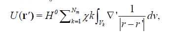(2)

All magnetic vector and tensor fields can be computed from the first and second spatial derivatives of equation 1, respectively. The second spatial derivatives of equation 1 form a symmetric magnetic tensor:

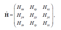(3)

with zero trace, implying that of the nine tensor components, only five are independent.

Closed-form solutions for the volume integrals over right rectangular prisms of magnetic susceptibility have been previously presented, e.g. [7]. In our implementation, we prefer to evaluate the volume integral numerically using single-point Gaussian integration with pulse basis functions [8].

Inversion

In a discrete form, similar to equation 2, the magnetic vector and tensor components can be written using the matrix equation:

d = Am (4)

where d is the N_d length vector of observed magnetic vector and/or tensor data, m is the N_m length vector of magnetic susceptibilities, and A is an N_d × N_m matrix of the linear forward modeling operator for magnetic vector and/or tensor fields. Various methods of compression may be introduced to minimize the storage of A(e.g., [9,10]). Inversion of equation 4 is ill-posed, and its solution requires regularization [11]. We can solve the linear inverse problem 4 using the Tikhonov parametric functional with a pseudo-quadratic stabilizer [5]:

P^α (m)=φ (m) +α s(m)→min, (5)

where φ (m) is a misfit functional:

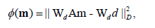(6)

And is a pseudo-quadratic stabilizing functional:

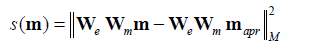(7)

Where W_d and W_m are the diagonal data and model weighting matrices, respectively. W_e is a diagonal matrix used to select a type of focusing stabilizing functional. In this paper, we use the minimum support (MS) stabilizer [5]:

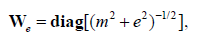(8)

which recovers models with sharp boundaries and contrasts, where e is a focusing parameter that is a small number chosen to avoid singularity in the stabilizer when m = 0. Equation 5 can be solved using a variety of optimization methods. For improved convergence and to avoid any matrix inversions, we minimize equation 5 using the re-weighted regularized conjugate gradient (RRCG) method [5].

In practical applications of the inversion method, some boundary conditions must be imposed on the variations of the model parameters:

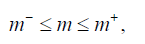(9 )

Where m^- and m⁺ are the lower and upper limits of the model parameter m. However, during the process of minimization of the Tikhonov parametric functional, we can get the values of the model parameters outside the above boundaries. In order to limit the interval of possible values of the inverse problem solution, one can introduce a new model parameter m′ with the property that the corresponding original model parameter m will always remain within the imposed above boundaries m^- and m⁺.One way to solve this problem is by using the following logarithmic transformation:

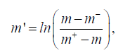(10)

with the corresponding inverse transformation:

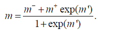(11)

It is obvious that the inversion is in the space of logarithmic model parameters m′, then no matter how large or how small the value of m will be, the inverse transformation by equation 11 will always keep the value of m exactly within the intervals formed by m^- and m⁺.

To investigate the performance of our 3D regularized inversion for both magnetic vector and tensor data, we considered two synthetic 3D models of dimensions typical for mineral exploration. In both cases, the magnetic vector data consisted of three vector components, and the magnetic tensor data consisted of all five independent tensor components. The first synthetic model represents of a rectangular body 60 m wide with a 10 m × 10 m of cross-sectional area, buried 30 m below the surface. The susceptibility of the body is 1, and it is embedded in an otherwise homogeneous and nonmagnetic host. The inducing magnetic field has an inclination of 90 degrees and a declination of zero degrees. Both magnetic vector and tensor data were contaminated with 5% random noise. The results are shown in Figure 1. As can be seen, the body is recovered from both vector and tensor data inversions. As expected, the latter provides a more compact image of the body.

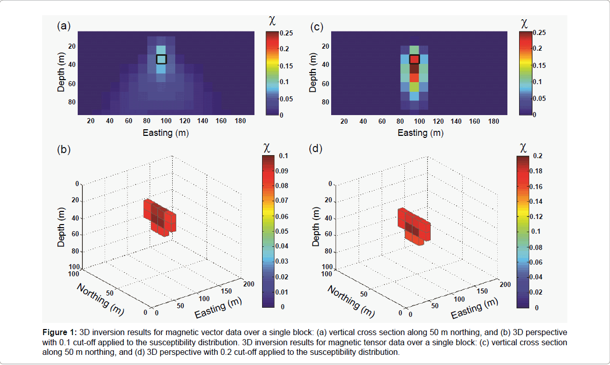
Figure 1: 3D inversion results for magnetic vector data over a single block: (a) vertical cross section along 50 m northing, and (b) 3D perspective with 0.1 cut-off applied to the susceptibility distribution. 3D inversion results for magnetic tensor data over a single block: (c) vertical cross section along 50 m northing, and (d) 3D perspective with 0.2 cut-off applied to the susceptibility distribution.

The second synthetic model consists of two rectangular bodies. The first body is 60 m wide, with a 10 m × 10 m cross-sectional area, and is buried 30 m below the surface. The second body is separated by 90 m from the first body, is 40 m wide, with a 10 m × 10 m cross-sectional area, and is also buried 30 m below the surface. The susceptibility of both bodies is 1, and they are embedded in an otherwise homogeneous and nonmagnetic host. The inducing magnetic field has an inclination of 90 degrees and a declination of zero degrees. The results are shown in Figure 2. As can be seen, the bodies were recovered from both vector and tensor inversions. Again, as expected, the latter provides a more compact image of both bodies.

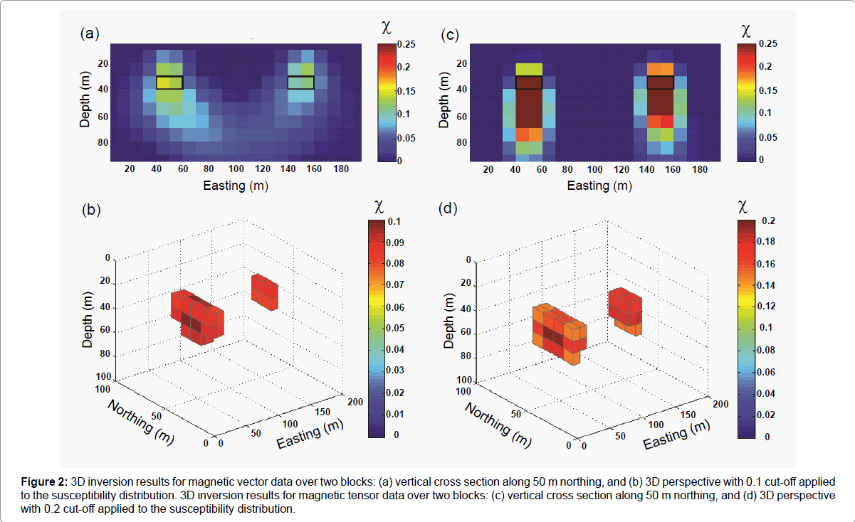
Figure 2: 3D inversion results for magnetic vector data over two blocks: (a) vertical cross section along 50 m northing, and (b) 3D perspective with 0.1 cut-off applied to the susceptibility distribution. 3D inversion results for magnetic tensor data over two blocks: (c) vertical cross section along 50 m northing, and (d) 3D perspective with 0.2 cut-off applied to the susceptibility distribution.

SQUIDS are the most appropriate sensors for measuring magnetic tensors as they detect minute changes of flux threading a superconducting loop. They are therefore variometers rather than magnetometers, but they are vector sensors since only changes perpendicular to the loop are detected [12-14]. CSIRO’s GETMAG system [1] is an integrated package of three rotating single-axial gradiometer sensors in an umbrella arrangement. This configuration has several distinct advantages [15]. First, it reduces the required number of sensors and electronics. Second, the amount of cross-talk between sensors is reduced by employing different rotation frequencies. This shifts the measurement (rotation) frequency from quasi-DC to tens or hundreds of hertz, leading to a reduced intrinsic sensor noise and a reduced influence of low-frequency mechanical vibrations; thus the requirements for suspension system during deployment are significantly reduced. Third, by implementing data extraction through Fourier analysis, magnetic vectors can be separated from magnetic tensors as the signals are centered at the fundamental and at twice the rotation frequency, respectively. Thus, with only three single-axial sensors, all vector and tensor components can be recovered.

The GETMAG system was demonstrated with a field trial of three profiles (50 mN, 60 mN, and 120 mN) over a magnetite skarn deposit at Tallawang, near Gulgong in New South Wales, Australia [1]. The deposit is roughly tabular, striking NNW and dipping steeply to the west. The survey was approximately perpendicular to strike, minimizing aliasing and effectively making the surveys 2D. The Tallawang magnetite skarn is located along the western margin of the Gulgong Granite, which was intruded during the Kanimblan Orogeny in the Late Carboniferous. The magnetite occurs in lenses thought to reflect replacement of a tightly folded host rock sequence, and is additionally complicated by transverse faulting causing east-west displacement of the magnetite zones. The magnetite body is well delineated by numerous drill holes, and the rock magnetic properties of the magnetite have been well characterised. The strongest samples possessed susceptibility of 3.8 SI (0.3 cgs) and remanence of 40 Am-1, yielding Köenigsberger ratios (Qs) between 0.2 and 0.5. The mean direction of the remanence is WNW and steeply up. This direction may be the result of a dominant viscous remanent magnetization in the direction of the recent geomagnetic field, and a reversed mid-Carboniferous component, dating from the time that the Gulgong Granite was intruded. The effective magnetization, projected onto a vertical plane perpendicular to strike, is directed steeply upward.

We applied our 3D regularized inversion to the three profiles of the GETMAG data to obtain 3D susceptibility models. First, we inverted the data using minimum support (focusing) regularization. For comparison, we then inverted the data using minimum norm (smooth) regularization. Both inversions terminated at a common misfit of 10%. Figures 3a to 3d show vertical and horizontal cross sections beneath each of the profiles and at 25 m depth as obtained from 3D inversion with focusing regularization. Figures 3e to 3h show vertical and horizontal cross sections beneath each of the profiles and at 25 m depth, as obtained from 3D inversion with smooth regularization. Both models satisfy the magnetic tensor data to the same misfit, yet we can clearly see how the focusing regularization enables us to recover much sharper boundaries and higher contrasts than smooth regularization. Moreover, as we superimposed the geology (Figure 4), we can see excellent agreement between our focusing inversion results and the known geology where we have sensitivity.

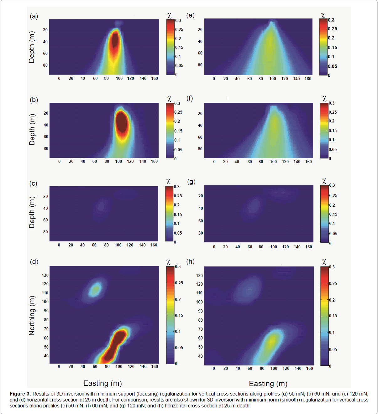
Figure 3: Results of 3D inversion with minimum support (focusing) regularization for vertical cross sections along profiles (a) 50 mN, (b) 60 mN, and (c) 120 mN; and (d) horizontal cross section at 25 m depth. For comparison, results are also shown for 3D inversion with minimum norm (smooth) regularization for vertical cross sections along profiles (e) 50 mN, (f) 60 mN, and (g) 120 mN; and (h) horizontal cross section at 25 m depth.

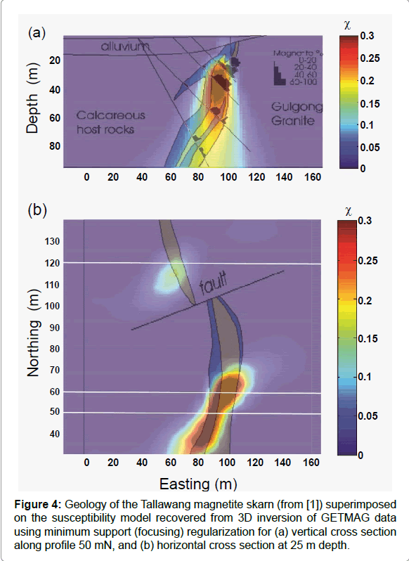
Figure 4: Geology of the Tallawang magnetite skarn (from [1]) superimposed on the susceptibility model recovered from 3D inversion of GETMAG data using minimum support (focusing) regularization for (a) vertical cross section along profile 50 mN, and (b) horizontal cross section at 25 m depth.

We have developed 3D regularized inversion for magnetic tensor data. Our model studies have shown that inversion of all independent magnetic tensor components can significantly improve model resolution compared to inversion of all magnetic vector components. We have applied our 3D regularized inversion to GETMAG magnetic tensor data acquired over a magnetite skarn at Tallawang in New South Wales, Australia. Our results agree very well with the known geology of the area, and show how magnetic tensor data can significantly improve the practical effectiveness of magnetic methods for exploration.

The authors thank TechnoImaging for support of this research and permission to publish. M. S. Zhdanov and H. Cai also acknowledge support of the University of Utah’s Consortium for Electromagnetic Modeling and Inversion (CEMI). The authors thank CSIRO Materials Science and Engineering, in particular Drs. Phil Schmidt, Keith Leslie, David Clark, and Cathy Foley, for providing the Tallawang GETMAG data and related material.