Journal of Geology & Geophysics
Open Access
ISSN: 2381-8719
ISSN: 2381-8719
Research Article - (2017) Volume 6, Issue 3
There is an insatiable thirst for oil and gas consumption and increased production will be made possible only through effective reservoir characterization and modeling. A suite of wire-line logs for four wells from ‘DEL’ oil field together with 3D seismic data were analyzed for reservoir characterization of the field. Two reservoirs were identified using the resistivity log. A synthetic seismogram was generated in order to perform seismic to well tie process as well as picking of horizons throughout the section. Time and depth structural maps were generated. Geostatistical simulation such as the sequential Gaussian stimulation and sequential indicator stimulation were carried out to provide equiprobable representations of the reservoirs, and the distribution of reservoir properties within the geological cells. The modeled reservoir properties resulted in an improved description of reservoir distribution and inter connectivity. The analysis indicated the presence of hydrocarbon in the reservoirs. There is also a fault assisted closure on the structural map which is of interest in exploration. A fluid distribution plot and map of the field were also obtained. The modeled properties gave an average porosity of 24%, average water saturation ranging from 12%-24% and moderate net-gross. The volumetric calculation of the reservoir gives a STOIIP ranging from 37.53 MMbbl-43.03 MMbbl. The result showed high hydrocarbon potential and a reservoir system whose performance is considered satisfactory for hydrocarbon production. The resulting models can also be used to predict the future performance of the reservoir.
Keywords: Porosity; Permeability; Reservoir characterization; Synthetic seismogram
The search for hydrocarbon is becoming increasingly more difficult and expensive. Because most of the identified structural closures on the shelf and upper slope have been drilled, the search for hydrocarbon and its production requires more creativity in optimizing and integrating existing data. The reservoir is the habitat of petroleum, and therefore an enhanced understanding of the reservoir will enable a proper prediction of its characteristics and requisite inputs for modeling. A reservoir that is well understood will ultimately result in a field that is well managed. Mapping the right reservoir, understanding of reservoir characteristics most importantly porosity, permeability, water-saturation, thickness and area extent of the reservoir so as to have a maximum hydrocarbon reserves have been a major challenge in the exploration and exploitation of hydrocarbon in major hydrocarbon fields within the world today such as Niger-Delta. Steady success in the exploitation for oil and gas reserves in Niger-Delta therefore depend on having a clear understanding about the subsurface geology of the area. The ability to accurately identify the fluid present within the reservoir, predict the petro physical parameters, model and estimate accurately the amount of reserves in the reservoir will aid in a successful exploitation for hydrocarbon.
In many cases, conceptual models are essential at the scale of the reservoir unit, but their accuracy commonly remains insufficient to realistically predict the distribution of internal heterogeneities [1]. Stochastic approaches are now more frequently applied to simulate the distribution of small-scale sedimentary bodies and internal reservoir heterogeneity [2-5]. Geostatistical approaches also provide equiprobable realizations of the heterogeneity distribution. This flexibility can be used to evaluate the impact of different geological scenarios, which contribute to the optimization of a field development plan. The advances in computational technology, modern reservoir models can accommodate increasingly detailed 3D data that illustrate the spatial distribution of reservoir properties. Subsurface reservoir characterization typically incorporates well data augmented with seismic data to establish the geological model of the reservoir [6]. A successful reservoir characterization therefore involves the integration of 3D seismic data and well log data. Integrating various datasets to provide a geologically relevant subsurface image will aid interpretation and reduce uncertainty. This is with the aim of delineating the subsurface structures that are favourable for the accumulation of hydrocarbon within the ‘DEL’ field and also to construct a fit for purpose geologic model.
Geology and location of the study area
Niger Delta is a prolific hydrocarbon belt in the world. The formation of Niger Delta basin was initiated in the early tertiary time. The Niger Delta is situated in the Gulf of Guinea and extends throughout the Niger Delta province [7]. From the Eocene to the present, the Delta has prograded Southwest ward, forming depobelts that represent the most active portion of the Delta at each stage of its development [8]. These depobelts form one of the largest regressive deltas in the world with an area of some 300,000 km2 a sediment volume of 500,000 km3 and a sediment thickness of over 10 km in the basin depocenter [9,10].
The Niger Delta province contains only one identified petroleum system [9,11]. This system is referred to here as the tertiary Niger Delta (Akata-Agbada) Petroleum System. Deposition of the three formations occurred in each of the five off lapping siliciclastic sedimentation cycles that comprise the Niger Delta. These cycles (depobelts) are 30-60 kilometres wide, prograde south-westward 250 kilometres over oceanic coast into the gulf of guinea and are defined by synsedimentary faulting that occurred in response to variable rates of subsidence and sediment supply [8,12].
The Delta formed at the site of a rift triple junction related to the opening of the Southern Atlantic starting in the late Jurassic from interbedded marine shale of the lower most Agbada formation and continuing into the cretaceous. The Delta proper began developing in the Eocene, accumulating sediments that now are over 10 km thick. The primary source rock is the upper Akata formation, the marine-shale facies of the Delta, with possibly contribution from interbedded marine shale of the lowermost Agbada formation. Oil is produced from sandstone facies within the Agbada formation, however, turbidite sand in the upper Akata Formation is a potential target in deep water offshore and possibly beneath currently producing intervals onshore. The intervals, however, rarely reach thickness sufficient to produce a world class oil province and are immature in various parts of the delta [12]. The Akata shale is present in large volumes beneath the Agbada Formation and is at least volumetrically sufficient to generate enough oil. Based on organic-matter content and its types, Evamy et al. proposed that both the marine shale (Akata Formation) and the shale interbedded with paralic sandstone (lower Agbada Formation) were the source rocks for the Niger Delta oils [13,14]. Petroleum occurs throughout the Agbada Formation of the Niger Delta, however, several directional trends form an "oil-rich belt" having the largest field and lowest gas:oil ratio [8,15]. The belt extends from the northwest off-shore area to the southeast offshore and along a number of north-south trends in the area of Port Harcourt. It roughly corresponds to the transition between the Continental and Oceanic crust and is within the axis of maximum sedimentary thickness.
This hydrocarbon distribution was originally attributed to the timing of trap formation relative to petroleum migration (earlier landward structures trapped earlier migrating oil), however, showed that in many rollovers, movement on the structure building fault and resulting growth continued and was relayed progressively southward into the younger part of the section by successive crestal faults [13]. He also concluded that there was no relation between growth along a fault and distribution of petroleum.
The study area (‘DEL’ FIELD) falls within the western margin of off-shore depobelt of Niger Delta (Figure 1). The fault pattern is NWSE and the traps involved in this field are mainly structural in nature. The study area is within the Parasequence set of Agbada formation. The field covers approximately 720 sq km.

Figure 1: Base map of ‘DEL’ field showing the well locations and seismic lines orientation.
Reservoir geology
The lithology was delineated by first setting a range for the gamma ray log. The gamma ray log ranges from 0 API to 150 API. The shale formations have high radioactive contents, thus deflecting to the right of the baseline while the sand formations will deflect to the left of the baseline since they have low radioactive content. Two reservoirs were correlated across the four (4) wells using both the gamma ray log and the resistivity log. The fluid types within these reservoirs were identified using both the neutron and density logs.
Seismic interpretation
Prominent geologic structures such as faults were identified across the seismic section. The check shot data from “DEL 4” was used to generate synthetic seismogram which was later used to tie the information from the well to our seismic data. The seismic events that correspond to the two reservoirs sand via the synthetic seismogram were mapped across the field. The mapped horizons were then contoured by the software to generate a structural time map. The check shot data shows a relationship between the two-way time (TWT) and True Vertical Depth (TVD) plotted against each other (Figure 2). A polynomial equation of the second order was derived from the plot. The equation was then used to build a velocity model which was used to convert the time structural map to depth structural map.

Figure 2: TWT-Z curve used for depth conversion using polymonial method.
Petrophysical evaluation
Volume of shale: The volume of shale within the reservoir was determined from the gamma ray log. This was achieved by first calculating the gamma ray index using the equation below:
 (1)
(1)
where: IGR=gamma ray index, GRLOG=gamma ray reading of the formation, GRMIN=minimum gamma ray (clean sand); GRMAX=maximum gamma ray (shale). The gamma ray index was then used to calculate the volume of shale using the Steiber equation [16].
 (2)
(2)
Total porosity: The total porosity gives the ratio of pore volume to the total volume of the reservoir. It was evaluated using the Wylllie equation [17].
 (3)
(3)
where: ρma=matrix density=2.684, ρb=formation bulk density, ρf=fluid density (1.1 salt mud, 1.0 fresh mud, 0.8 oil and 0.6 gas) and Φ=porosity
Effective porosity: The effective porosity gives the volume of the interconnected pore spaces within the reservoir i.e. it gives the volume of pore spaces that is contributing to the production of fluid within the reservoir. The effective porosity was evaluated using the equation below;
 (4)
(4)
Permeability: This gives the rate at which the fluid can move within the interconnected pore spaces [18].
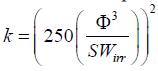 (5)
(5)
where: K=permeability, Φ=porosity and SWirr=irreducible water saturation.
Water Saturation: This was estimated using the Archie’s equation [19].
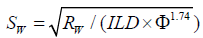 (6)
(6)
where SW=water saturation, RW=water resistivity and ILD=true resistivity
Static model
The first step in building a 3D geologic model is to construct a skeletal framework where both the discreet and continuous properties will be distributed into the geologic cells. This was done through a process called “pillar gridding”. Up scaling which is the process where values are assigned to the cells penetrated by the well logs in the 3D grid was also carried out. Since each cell can only hold one value, the well logs must be averaged, i.e., the lithology, resistivity, porosity, permeability, water saturation and EOD logs are up scaled into the 3D grid using the arithmetic mean method. The quality of the up scaled logs is checked by inspecting their histogram produced by the software. This is used for comparing the raw logs with the up scaled logs. If there is no much disparity between them, the up scaled logs are acceptable. Variogram analysis which is a function describing the degree of spatial dependence of a spatial random field or stochastic process was carried out. This variogram gives a measure of how data taking from the field varies in percentage depending on the distance between the data. Samples taking far apart will vary more than sample taking close to each other. The larger the separation distances between two points, the larger the variability. A variogram must be specified when a discrete property is “populated” (that is extrapolated to densely spaced points) using a stochastic simulation algorithm. The variogram analysis was carried out for all zones along the vertical direction. Cross plots which is also a statistical tools/ methods that provides the relationship between two variables was carried out. It was used to determine the relationship between some reservoir properties such as water saturation, permeability and effective porosity. These cross plots were later used as a secondary variable in the co-simulation technique.
The next step involves facies and property modeling. Facies and Property modeling is the distribution of reservoir rock properties into the 3D geocellular models using geostatistical principles. 3D property modeling without adequate data analysis will result into models that have little or no relation to geology. Therefore, a good knowledge about the geology of the area is needed to get meaningful property modeling. This is where the variogram analysis comes into play. Stochastic simulation which is a method of generating multiple equally probable realizations of reservoir properties was employed [20]. Sequential Indicator Stimulation (SIS) and Sequential Gaussian simulation (SGS), one of the dominant forms of stochastic simulation for reservoir modeling applications, was utilized. The algorithm was used to generate geologic models that honor the local conditioning (well) data, the global histogram, areal and vertical geological trends of the data and patterns of spatial correlation. The relationship between the water saturation and porosity also known as transformation plot was used to build the water-saturation model. The transformation plot was used to calculate for uncertainties within the reservoirs when the volumetric is been computed. The upper-case, base-case and low-case relationship between porosity and water-saturation was determined.
Reservoir geology
The well correlation of “Del” field was carried out along the strike. Four wells namely; DEL1, DEL2, DEL3, and DEL4 were correlated together along the strike direction (Figure 3). One of the major reasons for carrying out correlation exercise within the given wells is to have an idea of the occurrences of horizontal sand packages from one well to the other that were deposited at the same time and space within the field. It was observed from the correlation panel that the sand packages are thinning towards the N-E direction. Two reservoirs were identified within this field. They include; Reservoir B and Reservoir E.

Figure 3: Lithology delineation and well correlation.
The fluid types (oil and gas) within these reservoirs were identified using both the neutron log and density log respectively. It was observed that the wells within this field were saturated mostly with oil (Figures 4a and 4b).

Figure 4a: Reservoir identification in reservoir B.

Figure 4b: Reservoir identification in reservoir E.
Structural interpretation
One major fault was identified across the seismic section (Figure 5). Other faults identified within this field are synthetic and antithetic to the major fault. It was also observed from the seismic-well tie that the synthetic trace with the well tops also tie very well on the seismic section (Figure 6). From the structural time and depth maps of both reservoirs (Figures 7 and 8), it was observed that the maps are having an anticlinal structure (four-way dip closure) which is of importance to the petroleum geologist, geophysicists and engineers since hydrocarbon do accumulate within an anticlinal structure. The direction of the major fault is along the NW-SE. The other faults within this field are either synthetic or antithetic to the major faults. It was also observed from the elevation legend that the orange color indicates the shallowest part of the field while the green color indicates the deepest part of the field. The closure within this field is a fault assisted closure which serves as a seal that prevented further migration of hydrocarbon.

Figure 5: Fault mapped on the seismic section.

Figure 6: Seismic to well tie.

Figure 7: Structural time map and depth map for reservoir.

Figure 8: Structural time map and depth map for reservoir E.
Static model
From the result, it was observed that the top, mid, and base skeleton (Figure 9) serve as the structural framework for reservoir modelling. The skeleton frame work of the reservoir has total grid cells of 323,850. This implies that the geological heterogeneities will be captured with grid resolution for the construction of a fit for purpose geological model. From the petrophysical parameters evaluated for both reservoirs, it was observed that much hydrocarbon can be economically exploited from both reservoirs due to their high porosity and low water saturation. Based on this, 3D geologic model was constructed for reservoir E so as to know how these properties are being distributed within the subsurface. The total porosity and effective porosity which is a continuous properties of the reservoir was distributed properly within the geologic cells of the reservoir E ad modeled. The total porosity gives the ratio of pore volume to the total volume of the reservoir. The total porosity model shows that reservoir E has a minimum porosity of 0.16 and a maximum porosity of 0.30 (Figure 10). The model shows that the reservoir has an average total porosity of 24%. (Figure10). These indicate that the reservoir is very porous and well completed.

Figure 9: Pillar gridding showing the top, mid and base skeletal frame work of the static model.

Figure 10: Porosity model for reservoir E.
From the colour legend, areas with very low porosity are indicated by the purple colour while areas with high porosity are indicated with orange colour. The effective porosity gives the volume of the interconnected pore spaces within the reservoir i.e. it gives the volume of pore spaces that is contributing to the production of fluid within the reservoir. The effective porosity model shows that reservoir E has a minimum effective porosity of 0.07 and a maximum effective porosity of 0.28. The average effective porosity within this reservoir is 0.22. These indicate that the pore spaces within the reservoir are well connected. The permeability model (Figures 11a and b) indicate that the rate of flow within the reservoir is high.

Figure 11a: Cross plot of porosity against permeability.

Figure 11b: Permeability model for reservoir E.
From the transformation plot (Figure 12a); three different water saturation cases were identified. These include the base case water saturation, low case water saturation, and high case water saturation. The low case water saturation model gives an average water saturation of 0.23, while the high case water saturation model gives an average water saturation of 0.12. This implies that a lot of hydrocarbon can be exploited at the high case than the low case water saturation. The water saturation model for the base case shows that reservoir has a minimum water saturation of 0.06 and a maximum water saturation of 0.38 (Figure 12b). The average water saturation within this reservoir is 0.23. These indicate that the reservoir is 0.77 saturated with hydrocarbon. Areas with blue colour indicate part of the reservoir that is completely saturated with water.

Figure 12a: Transformation plot for reservoir E.

Figure 12b: Water saturation for reservoir E using the base-case.
Volumetric Analysis
STOIIP=GRV × POROSITY × NTG × (1-SW) / BO
This research work shows the versatility of integrating 3D seismic reflection, and well logs data for interpretation, petro physical analysis and construction of a 3D geologic model. The accumulation and trapping of hydrocarbon in this field is fault assisted. Reservoirs B &E are very promising because of its very good porosity values, low water saturation, high hydrocarbon saturation (SH), good permeability and moderate net to gross. The static model of reservoir E indicate that the reservoir has an average total porosity of 24% (Table 1), effective porosity of 22%, water saturation ranging from 12%-23% (Table 1) and permeability of 4476 mD. The volumetric calculation indicates that Reservoir E has a STOIIP ranging from 37.53-43.03 × 10^6 STB (Table 1) respectively.
| GRV (FT) | POROSITY | NTG | SW | HS | STOIIP (MMBL) | |
|---|---|---|---|---|---|---|
| 950356 | 0.24 | 0.67 | 0.17 | 0.83 | 40.84 | BASE-CASE |
| 950356 | 0.24 | 0.67 | 0.23 | 0.77 | 37.53 | LOW-CASE |
| 950356 | 0.24 | 0.67 | 0.12 | 0.88 | 43.03 | HIGH-CASE |
Table 1: Summary of volumetric analysis for reservoir E from 3-D model.
Further interpretation such as Seismic attribute analysis, AVO analysis, Seismic inversion, Rock physics, etc. should be carried out on the field so as to affirm the existence of hydrocarbon and the tapping mechanism in this field. Uncertainty analysis such as Monte Carlo stimulation, material balance analysis, etc. should also be used to evaluate and affirm the STOIIP value. This will help to affirm if the field is economically fit for exploitation. More wells should be drilled along the west and east direction of the field. This will help in the proper optimization of the field.
Our appreciation goes to Integrated Data Services Limited, Benin-City, Nigeria for releasing the data used to carry out this research work.