


Indexed In
- Open J Gate
- RefSeek
- Hamdard University
- EBSCO A-Z
- OCLC- WorldCat
- Publons
- International Scientific Indexing
- Euro Pub
- Google Scholar
Useful Links
Share This Page
Journal Flyer

Open Access Journals
- Agri and Aquaculture
- Biochemistry
- Bioinformatics & Systems Biology
- Business & Management
- Chemistry
- Clinical Sciences
- Engineering
- Food & Nutrition
- General Science
- Genetics & Molecular Biology
- Immunology & Microbiology
- Medical Sciences
- Neuroscience & Psychology
- Nursing & Health Care
- Pharmaceutical Sciences
Research Article - (2020) Volume 9, Issue 2
Shift Estimation for DMSP-OLS Night-Time Light Rasters in 2009âÂÂ2011
Geng X1, Xue S1, Yan XH2,3*, Xie T1,3,4 and Huo C52Center for Remote Sensing, College of Earth, Ocean and Environment, University of Delaware, Newark, DE 19716, China
3Joint Institute for Coastal Research and Management (Joint-CRM), University of Delaware/Xiamen Unive, USA/China Newark, DE 19716, USA/Xiang-An, Xiamen 361005, China
4Fujian Engineering Research Center for Ocean Remote Sensing Big Data, Xiamen 361005, China
5Science and Technology on Electromagnetic Scattering Laboratory, Beijing 100854, China
Received: 06-Apr-2020 Published: 27-Apr-2020, DOI: 10.35248/2469-4134.20.9.273
Abstract
Night-time lights in satellite imagery are considered to be related to population and human activities such as urbanization, energy consumption, and CO2 emissions. The Defense Meteorological Satellite Program (DMSP) Operational Line-Scan System (OLS) instrument has provided a long-term dataset of global night lights covering more than two decades. However, the F162009, F182010, and F182011 rasters of DMSP-OLS version 4 night-time lights time series are shifted for unknown reasons, which may influence spatial time series comparisons. This study presents a statistical correlation method based on fast Fourier transform (FFT) to estimate these shifts in longitude and latitude with greater accuracy, and recommends the use of them to generate the accompanying Tiff World (TFW) files of tiff images for these rasters.
Keywords
Night-time lights; Remote sensing; Defense Meteorological Satellite Program (DMSP); Operational Linescan System (OLS)
Introduction
Remote sensing of night-time lights is an important tool for monitoring human activity from space [1]. This is especially true for data related to population and social economic activities such as urbanization, energy consumption, and CO2 emissions [2-5]. From the Defense Meteorological Satellite Program (DMSP) Operational Line-scan System (OLS) to the Suomi National Polar-Orbiting Partnership (NPP) Visible Infrared Imaging Radiometer Suite (VIIRS) Day/Night Band (DNB), a growing number of night-time lights products are being provided. In June 2018, the Luojia 1-01 (LJ1-01), a new custom-designed satellite for remote sensing of night-time lights was launched [6].
Moststudies of night-time lightsrelated to human activity need dynamic analysis, but varying atmospheric conditions, satellite shifts, and sensor degradation mean that the digital number (DN) of night-time lights data cannot be directly used for dynamic detection [7]. Therefore, the geometry and radiation calibrations of the data are crucial for such applications. The DMSP-OLS offers a unique long-term global night lights dataset that covers more than two decades. However, for some unknown reasons[8], the F162009, F182010, and F182011 rastersare shifted. Additionally, there are no accompanying Tiff World (TFW) files of tiff images for these rasters, which may influence spatial time series comparisons. It has been reported that this shift was half a pixel [8] and the nearest neighbor method was adopted to resample the three rasters to match the extent of other data while preserving their values.
These shifts have been ignored or simplified in most related research; however, this study will present a statistical correlation method based on fast Fourier transform (FFT) to estimate longitude and latitude shifts, and recommend the results to be adopted to generate more accurate TFW files for these rasters. Section 2 describes the data and the method in detail, Section 3 presents the proposed method’s results, and Section 4 provides a discussion and conclusions.
Data And Methods
Data
The DMSP satellite constellation has been in operation since the 1960s to observe clouds and other weather variables for weather forecasters [9]. The first DMSP-OLS sensor, an oscillating scan radiometer with low-light visible and thermal infrared (TIR) imaging capabilities, was flown in 1976. This instrument was designed to detect smoke and dust storms, and was uniquely sensitive to view clouds by moonlight. It was soon found that DMSP-OLS could also capture city lights and fires [10], which initiated remote sensing of night-time lights. Since the 1970s, almost 20 DMSP satellites carrying OLS and other types of sensors were launched. These satellites fly in sunsynchronous polar orbits with an altitude of 840 km and period of 101 minutes. There were always several DMSP satellites around the Earth simultaneously, and these satellites had collected the longest-term dataset of global night-time nights.
The DMSP-OLS version 4 night-time lights time series, provided by the National Centers for Environmental Information (NCEI) of National Oceanic and Atmospheric Administration (NOAA), consists of 34 annual composites from six satellites (F10, F12, F14, F15, F16, and F18) spanning 22 years (1992-2013)[11]. These data are cloud-free composites of all available archived DMSP-OLS smooth resolution data for those calendar years and have a grid of 30 arc-seconds (approximately 1 km at the equator) and span -180 to 180 degrees longitude and -65 to 75 degrees latitude. Each file contains a total of 725,820,001 pixels arranged in 16,801 rows and 43,201 columns. Figure 1 shows the F18 2013 stable night-time lights composite as an example.

Figure 1. Stable night-time lights compositeof F18 2013.
This dataset does not have accompanying TFW files for the F162009, F182010, and F182011 rasters, which are shifted for unknown reasons. To properly study the night-time lights in a spatial time series related with social and economic activities, these longitude and latitude shifts should be accurately estimated.
Method
The proposed method is motivated by work on Doppler frequency estimation for synthetic aperture radar of Bamler [12], and utilizes the principle of energy balancing based on statistical correlation along rows and columns to estimate respective longitude and latitude shifts, while choosing another raster with the TFW file as a reference. Here we demonstrate the longitude shift estimation process for a raster as an example.
At first, the summations of each column in the target and referenced rasters are calculated as follows:
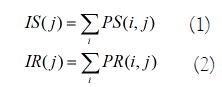
Where i and j denote the number of rows and columns, respectively, PS is the target raster, and PR is the referenced raster. This operation reduces the latitude dimension, which will make the longitude shift estimation more accurate.
Because the shift value in pixels may not be an integer, we use an interpolation method based on a discrete Fourier transform with zero-padding [13] to produce a better estimation. Thus, the summations IS and IR must be transformed to the frequency domain through FFT, which can be expressed as:
SS=FFT[IS] (3)
SR=FFT[IR] (4)
Then, zero-padding is applied at the beginning and end of the two spectra:
SSZ=[0,…,0,SS(1),…,SS(43201),0,…,0] (5)
SRZ=[0,…,0,SR(1),…,SR(43201),0,…,0] (6)
In Eqs. (5) and (6), the numbers of zeros for padding on the left and right are determined by the interpolated time K, and can be expressed as (K˗1)*43201/2.
Next, we transform SSZ and SRZ back to the space domain using an inverse FFT (IFFT):
ISZ(n)=IFFT[SSZ(n)] (7)
IRZ(n)=IFFT[SRZ(n)] (8)
The key step here is to calculate the correlation between ISZ and IRZ, which in principle is circle convolution and could be improved using FFT and IFFT for computation efficiency:
C(n)=|IFFT{FFT(ISZ) . conj[FFT(IRZ)]}| (9)
In Eq. (9), conj denotes the complex conjugate operation. Thus, as we attempt to find the shift, a circle convolution of IRZ and itself is also required:
Cr(n)=|IFFT{FFT (IRZ) . conj[FFT(IRZ)]}| (10)
Assuming that nc and ncr are the locations of maximum values in C(n) and Cr(n), respectively, the shift can then be estimated as:.
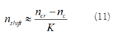
Figure 2 shows the block diagram of the proposed method for shift estimation. In this study, we assigned K a value as 11 and used the mean of the rastersF162008 and F182012 as the reference raster to estimate the shifts in the F162009, F182010, and F182011rasters. Because the coordinate information in the F162008 and F182012 TFW files are slightly different, the latter had to be interpolated to keep same coordinates as the former.

Figure 2. Block diagram of the shift estimation method.
Results and Discussion
Figures 3 and 4 show the summations of intensity along latitude and longitude after interpolation, respectively. These summations were used to estimate shifts of less than one pixel. The red curves indicate the reference raster, whereas the blue curves represent the target rasters.

Figure 3. Summations of intensity along latitude after interpolation.

Figure 4. Summations of intensity along longitude after interpolation.
The shift estimation results are shown in Table 1, with positive values indicating a rightward or downward shift and negative values representing a leftward or upward shift. Based on these results, the shifts of the F162009 raster are approximately half a pixel as described in [8]; however, they are shifted leftward in the columns and downward in the rows. For the F182010 raster, the leftward shift in the columns is the highest (1.27), whereas the downward shift in the rows is miniscule(-0.09). Lastly, the shifts of the F182011 raster are relatively small.
To validate the proposed method, two experiments were conducted, and their results are provided in Tables 2 and 3, respectively.
In these experiments, we assumed there were no accompanying TFW files for the F162005, F162006, F162007, and F182013 rasters, and then we used the proposed method to estimate their shifts and compared those results with the corresponding TFW files.
In the first experiment, we selected the means of rasters F162008 and F182012 (Table 1) as the reference raster; however, for the other experiment we used rasters near the target raster’s year as the reference raster. As there is no TFW file in F162009, only raster F162007 was used as the reference raster for F162008 in Table 2.
| Raster | F162009 | F182010 | F182011 |
|---|---|---|---|
| Columns Shift | −0.64 | −1.27 | 0.27 |
| Rows Shift | 0.55 | 0.09 | 0.36 |
| Estimated Longitude | −179.9947 | −179.9894 | 180.0023 |
| Estimated Latitude | 75.0046 | 75.0008 | 75.003 |
Table 1: Shift estimation results.
| Target Raster | F162005 | F162006 | F162007 | F182013 |
|---|---|---|---|---|
| Reference Raster | F162008 | F162008 | F162008 | F162008 |
| F182012 | F182012 | F182012 | F182012 | |
| Columns Shift | −0.45 | −0.72 | −0.36 | −0.09 |
| Rows Shift | −0.18 | 0 | −0.18 | 0 |
| Longitude in TFW | −180.0000 | −180.0000 | −180.0000 | −180.0000 |
| Latitude in TFW | 75 | 75 | 75 | 75 |
| Estimated Longitude | −179.9963 | −179.9940 | −179.9970 | −179.9992 |
| Estimated Latitude | 74.9985 | 75 | 74.9985 | 75 |
| Latitude Error | 0.0037 | 0.006 | 0.003 | 0.0008 |
| Longitude Error | −0.0015 | 0 | −0.0015 | 0 |
Table 2: First experiment results (Longitude and latitude correspond to the top left pixel in a raster).
The differences between the estimated results and TFW files are relatively larger in Table 3, especially for the F162006 (shift: -0.72), F162005 (shift: -0.45), and F162007 (shift: -0.36) rasters, as the pixel resolution is only 30 arc seconds. However, almost all the shifts in Table 3 are less than one-fourth of a pixel, thus these errors of the proposed method could be ignored.
| Target Raster | F162005 | F162006 | F162007 | F162008 |
|---|---|---|---|---|
| Reference Raster | F162004 | F162005 | F162006 | F162007 |
| F162006 | F162007 | F162008 | ||
| Columns Shift | 0.18 | −0.27 | 0 | 0.18 |
| Rows Shift | −0.18 | 0.18 | −0.09 | 0.09 |
| Longitude in TFW | −180.0000 | −180.0000 | −180.0000 | −180.0000 |
| Latitude in TFW | 75 | 75 | 75 | 75 |
| Estimated Longitude | −180.0015 | −179.9978 | −180.0000 | −180.0015 |
| Estimated Latitude | 74.9985 | 75.0015 | 74.9992 | 75.0008 |
| Latitude Error | −0.0015 | 0.0022 | 0 | −0.0015 |
| Longitude Error | −0.0015 | 0.0015 | −0.0008 | 0.0008 |
Table 3: Second experiment results (The longitude and latitude are corresponding the top left pixel in a raster).
Conclusion
Although the DMSP-OLS version 4 night-time lights time series has been widely used for night-time lights remote sensing applications, the F162009, F182010, and F182011 rasters have no accompanying TFW files, and their shifts are believed to be half a pixel. In this paper we presented an FFT-based statistical correlation method to estimate the shifts, which show different distributions. Additionally, we performed two experiments to validate the proposed method.
The processes for longitude and latitude shift estimation for a raster should be performed independently as the statistical correlations are related to the summation of each column or row. Even if the night-time lights change over time, the summations of columns and rows should maintain some consistency in the neighbor years, which ensures the proposed method’s feasibility. Based on the results in Table 1, TFW files with much greater accuracy could be generated for these rasters.
Author Contributions
Conceptualization, Xupu Geng and Xiao-Hai Yan; Formal analysis, ChaoyingHuo; Funding acquisition, Xiao-Hai Yan; Methodology, Xupu Geng and SihanXue; Software, SihanXue and ChaoyingHuo; Validation, Xupu Geng and Ting Xie; Writing- original draft, Xupu Geng and SihanXue; Writing - review & editing, SihanXue, Xiao-Hai Yan, Ting Xie and ChaoyingHuo.
Funding
This research was funded by the Open Research Fund of the State Key Laboratory of Information Engineering in Surveying, Mapping, and Remote Sensing, Wuhan University (18T08); the SOA Global Change and Air-Sea Interaction Project (grant numbers GASI-02-PAC-YGST2-02 and GASI-IPOVAI-01-04); and the National Natural Science Foundation of China (grant numbers 91858202 and 41906184).
Acknowledgment
The authors would like to thank NOAA for providing the DMSP-OLS version 4 night-time lights time series data.
REFERENCES
- Levin N, Kyba C, Zhang Q. Remote sensing of night lights-beyond DMSP. Rem Sens. 2019;11(12):1472.
- Sun W, Zhang X, Wang N, Cen Y. Estimating population density using DMSP-OLS night-time imagery and land cover data. IEEE J Selected Topics in App Earth Obs and Rem Sens. 2017:10(6):2674-2684.
- Gao B, Huang Q, He C, Ma Q. Dynamics of urbanization levels in China from 1992 to 2012: Perspective from DMSP/OLS nighttime light data. Rem Sens. 2015;7(2):1721-1735.
- Xie Y, Weng Q. World energy consumption pattern as revealed by DMSP-OLS nighttime light imagery. GI Sci & Rem Sens. 2016;53(2):265-282.
- Shi K, Chen Y, Yu B, Xu T, Chen Z, Liu R, et al. Modeling spatiotemporal CO2 (carbon dioxide) emission dynamics in China from DMSP-OLS nighttime stable light data using panel data analysis. App Energy. 2016;168:523-533.
- Li X, Zhao L, Li D, Xu H. Mapping urban extent using Luojia 1-01 nighttime light imagery. Sensors. 2018;18(11):3665.
- Li X, Zhou Y. A stepwise calibration of global DMSP/OLS stable nighttime light data (1992–2013). Rem Sens. 2017;9(6):637.
- Stathakis D. Intercalibration of DMSP/OLS by parallel regressions. IEEE Geo sci and Rem Sens Lett. 2016;13(10):1420-1424.
- Miller SD, Mills SP, Elvidge CD, Lindsey DT, Lee TF, Hawkins JD. Suomi satellite brings to light a unique frontier of nighttime environmental sensing capabilities. Proc of Nat Acad of Sci. 2012;109(39):15706-15711.
- DMSP (Defense Meteorological Satellite Program). Available online: https://directory.eoportal.org/web/eoportal/-/dmsp. (accessed on 20 October 2019)
- Version 4 DMSP-OLS Nighttime Lights Time Series. Available online: https://ngdc.noaa.gov/eog/dmsp/downloadV4composites.html. (accessed on 10 October 2019)
- Bamler R. Doppler frequency estimation and the Cramer-Rao bound. IEEE Trans on Geosci and Rem Sens. 1991:29(3):385-390.
- Fu-bin ZJXC, Qiang SZGF. Interpolation Algorithm for Discrete Fourier Transform with Zero-Padding. Sig Proc. 2007;5:293
Citation: Geng X, Xue S, Yan XH, Xie T, Huo C (2020) Shift Estimation for DMSP-OLS Night-Time Light Rasters in 2009-2011. J Remote Sens GIS. 9:273. DOI: 10.35248/2469-4134.20.9.273
Copyright: © 2020 Geng X, et al. This is an open-access article distributed under the terms of the Creative Commons Attribution License, which permits unrestricted use, distribution, and reproduction in any medium, provided the original author and source are credited.