

Indexed In
- Open J Gate
- Genamics JournalSeek
- Academic Keys
- ResearchBible
- Cosmos IF
- Access to Global Online Research in Agriculture (AGORA)
- Electronic Journals Library
- RefSeek
- Directory of Research Journal Indexing (DRJI)
- Hamdard University
- EBSCO A-Z
- OCLC- WorldCat
- Scholarsteer
- SWB online catalog
- Virtual Library of Biology (vifabio)
- Publons
- Geneva Foundation for Medical Education and Research
- Euro Pub
- Google Scholar
Useful Links
Share This Page
Journal Flyer

Open Access Journals
- Agri and Aquaculture
- Biochemistry
- Bioinformatics & Systems Biology
- Business & Management
- Chemistry
- Clinical Sciences
- Engineering
- Food & Nutrition
- General Science
- Genetics & Molecular Biology
- Immunology & Microbiology
- Medical Sciences
- Neuroscience & Psychology
- Nursing & Health Care
- Pharmaceutical Sciences
Research Article - (2019) Volume 8, Issue 1
Performance Analysis of Regression-Machine Learning Algorithms for Predication of Runoff Time
Marwan Khan1* and Sanam Noor22Institute of Business and Management Sciences/ Computer Science, University of Agriculture, Peshawar, Pakistan
Received: 05-Feb-2019 Published: 07-Mar-2019, DOI: 10.35248/2168-9881.19.8.187
Abstract
Worldwide 70 percent of water is used in agriculture practices, in which 50% of water is lost due to improperly planned and inefficient irrigation system. Precision irrigation system has long been used on individual farms scale. Very rare work has been done so far to utilize the excessive irrigation water of one farm in another farm. In this research, we address the problem of predicting the runoff time between two farms. We propose Runoff time model which accepts irrigation depth, soil moisture and crop stage (CN) and time of concentration as input parameters and estimate runoff time. Machine learning algorithms i.e., Multiple Linear Regression (MLR), Artificial Neural Network-Levenberg Marquardt (LMA-ANN), Decision Trees/Regression Tree (DT/RT) and Least Square Support Vector Regression (LS-SVR) have been used for learning and predication purposes. A comparison has been made among these algorithms to choose best algorithm for irrigation runoff time prediction. Experimental results show that regression tree aces the results in terms of highest R-square value, lowest Mean square error. While MLR shows the worse result in terms of least R-square value, highest means square error. The algorithms Regression tree is ranked first-outstanding, ANN-LMA is ranked second-good, LS-SVR is ranked third-fair and MLR is ranked last-poor on the basis of the regression error metrics/ performance evaluation parameters. Hence it is strongly suggested that regression tree is an ideal machine learning-regression algorithm to be deployed on the Wireless Sensor Network (WSN) node for the predication of runoff time.
Keywords
Wireless Sensor Network (WSN); Precision irrigation; Machine learning algorithms; Regression; Irrigation runoff time modeling
Introduction
With the growth in population, the water scarcity is increasingly becoming a more daunting factor in many parts of the world. Currently, the human population of the planet earth is estimated to be 6.8 billion and it is predicted to grow to 9.1 billion by 2050. With the rise in population, the demands for food also grow to 70 percent of the current demand. Hence, the steps must be taken to modernize and expand the agriculture, which requires more water and cultivable land. Although, Food and Agricultural Organization (FAO) projects that by 2050, the global cultivable land can be expanded to 70 million hectares, the scarcity of water in increasing number of countries can become a bottleneck in meeting the goals of sufficient food production. If the situation continues unabated, the scarcity of water would emerge as the biggest threat to the social and economic progress of many developing countries. Although water can be treated as a renewable source, in some parts of the world, its resources are either so heavily exhausted or polluted that it has hobbled the growth. The developing countries are facing the brunt of this crisis, where 95% of the new population is being spawned [1-3].
One of the sectors, which faces the brunt of water shortage, is the agriculture. As one of the most demanding sectors in agrarian societies, the shortage of water directly translates into decrease in the food production per capita [4]. Water mismanagement and primitive methods of cultivation have led to the sharp decrease in water resources; the most important of all is the traditional method of irrigation also known as “Surface Irrigation” or “Flood Irrigation” [5,6]. Due to poor efficiency of this method, an improperly designed flood irrigation causes a 40 to 60 percent loss of water in the form of runoff [7]. In order to maintain the production capacity, the need is to switch towards more efficient means of using the water, which can maximize the economic and social gains while using the minimum resources. This is possible through special efforts directed at enhancing equity in access and optimum allocation of water resources [8]. Water use efficiency, which can be defined as “yield generated per unit precipitation and/ or irrigation of water applied”, is the first determinant of the crop yield under conditions of water scarcity. One possible solution (and now widely used) is the process of recycling the wastewater for agricultural, domestic and industrial use. A large number of studies are now dedicated to the recycling water techniques. Another solution is the use of precision irrigation system which could be implemented at micro level on a farm land. Precision irrigation system uses wireless sensors network for data collection such as soil moisture, crop properties, temperature and humidity of a farm and either send the gathered data to data aggregator (gateway node) or could process the data collected by its own (node level) to make efficient decision making regarding how much water is required by the farm to be applied and when? As reported by Pacific Institute, “precision irrigation” can save water in irrigation from 11 percent to 50 percent [9].
Precision irrigation is used on individual farms. Very rare has been done so far to utilize the excessive irrigation water of one farm in another farm. There are usually a number of farms in the same vicinity. Some of them might be at a slightly higher ground level than others. If there are two farms next to each other, one at slightly higher level, then with proper planning and communication, excess water from the irrigation at the higher farm can be directed to irrigate the farm at the lower level. This method will have a twofold advantage. Firstly, water would be provided to the second farm in some span of time without actually having to utilize any surplus amount, other than that provided to the first one. Secondly, the extra amount of water provided to the first farm would be redirected away from it. This will prevent over watering of the crops. To counter this issue, a unique two-farm infrastructure, which can handle both these issues, is proposed.
Wireless Sensor Network (WSN) and precision irrigation system such as sprinklers deployed on an individual farms scale to save water is reactive rather than proactive. A proactive, intelligent and integrated irrigation water management and monitoring system is required on multiple farms to preserve water resources. This irrigation water management and monitoring system can be established by concatenating multiple farms in some geographic vicinity. In this study, a two-farm scenario has been considered; the approach that could be used is distributed rather than centralized. Whenever an irrigation event information occurs in farm A, WSN system installed on farm A has the capability to opportunistically connect with other neighbouring farm B in the same geographic vicinity to exchange the irrigation event information with farm B. This approach will allow to detect the irrigation event information and the sensors installed on farm A will be able to make predictions that when the outcome of that event might be seen on farm B. This will help in decision making on farm B to adjust its local farm irrigation objectives. The predictions to be performed by the sensors on the farm are required to have low complexity machine learning algorithms. The reason for that is because wireless sensor nodes have low battery power, computational power and absence of suitable sensors require a simplified machine learning models to be run on the sensor nodes. The WSN sensor node must be configured such that it has the capability of the acquiring the data in real time for the dynamic parameters (irrigation depth soil moisture and crop stage) and also to run the sophisticated machine learning algorithms to predict the farm A hydrological discharge amount and its time taken into another farm B.
This paper address the issue of prediction of irrigation runoff time from one farm to another. Different machine learning algorithms are tested and evaluated using different performance matrices. A comparison has been made among these algorithms. Further it is suggested that which algorithm will be ideal to deploy in real world on the sensor node level or on the gateway level on the WSN of the farm.
The remaining paper is organized as follow. Section 2 describes related work on precision irrigation and the role of machine learning algorithm for runoff modeling. Section 3 describes methodology. Section 4 presents discussion on methods and result. Finally section 5 concludes the paper.
Related Work
WSN has opened up new opportunities in environmental monitoring, precision agriculture, precision irrigation and hydrology. WSN is utilized in precision irrigation by monitoring soil moisture content to minimizing water wastage. Beside soil moisture other parameters like Leaf Wetness, Temperature and Relative Humidity, plant root depth, Sand Texture, Water Storage Capacities of Soil, Plant Water Use Capabilities can be monitored for efficient use of irrigation process [7]. Goumopoulos et al. [10] Describes an autonomous closed-loop zone-specific irrigation system based on the integration of WSN and adaptable decision based system. The proposed system control and monitor the irrigation process and plant growth in real time and is organized in a layered modular way to make it more flexible. The decision support system is able to learn by monitoring soil, crop and climate in a field and provides treatments, such as irrigation, to specific parts of a field in real time and proactively. In the similar context Mohapatra and Kumar [11] proposed neural network pattern classification technique for the forecast of soil Moisture Content (MC) by considering soil and environmental parameters. The predicated soil Moisture Content (MC) is used for creating appropriate notifications using fuzzy logic based weather model to generate irrigation recommendation.
Soil moisture is one key parameter for efficient water management and precision irrigation. Temporal variability analysis could be used to analyze soil moisture variations at different times of one day or between different days. Zhang et al. [12] Integrate WSN with spatial analysis software to monitor soil moisture and to do water saving and variable irrigation. Moisture sensors were placed at predetermined location in a field. The system sent the data of soil moisture periodically to the remote system. During the experimental period, the data of soil moisture were dynamically stored, and analysis of the temporal and spatial variability was performed in order to determine whether irrigation was required or not.
Machine learning is a very rich field and can be used for a variety of tasks such as classification, regression, bioinformatics, machine vision, fraud detection. Machine learning has been used in WSN and precision agriculture for decades. Integrating Machine learning with weather and soil data can be beneficial for water management and scheduling irrigation in agriculture fields. Machine learning can be used for creating prediction model for precision irrigation. In their work Navarro-Hellin et al. [13] proposed an automatic Smart Irrigation Decision Support System, SIDSS to forecast the weekly irrigations needs of crops. The main features is the use of continuous soil measurement with the climatic parameters to precisely estimate the irrigation requirements of the crops. It not only takes decision on the basis of weather variables but also take into account the quantity of water required by the crops.
Wan [14] Implement the precision irrigation system by employing machine learning, to find the accurate water demand of crop at different growth cycle of crop. The system consist of sensors nodes for measuring three parameters; humidity, soil moisture and irrigation volume. On basis of these three parameters machine learning model is built for predicting water requirements of crop and their growth status.
Soil Conservation Service Curve Number (SCS-CN) is one of the most popular and simplest hydrological models. It has renamed as the Natural Resource Conservation Service (NRCS) curve number method [15]. This method is used to estimate the volume of direct surface runoff and, its response and travel times for a given rainfall event. This method is used widely and is accepted in numerous hydrologic studies. The SCS method originally was developed for agricultural watersheds in the mid-western United States; however it has been used throughout the world far beyond its original developers would have imagined.
Hydrological models provide us a wide range of significant applications in the multi-disciplinary water resources planning and management activities. Soil water distribution and variation are helpful in predicting and understanding various hydrologic processes, including weather changes, rainfall/runoff generation and irrigation scheduling. Soil water content prediction is essential to the development of advanced agriculture information systems. Soil moisture is an integral variable in hydrology. Soil moisture information is critically important for many application areas such as irrigation scheduling, rainfall/runoff generation processes, reservoir management, crop yield forecasting meteorology, climate investigations, and natural hazards predictions. Prior knowledge of soil water content behaviour can not only help in better management and understanding of hydrological systems but also result in improved forecasting, especially in precision irrigation.
From literature, it is clear that there are various machine-learning algorithms used in the prediction of hydrological discharges [16]. Over the past several years, various attempts have been made to produce soil water content estimates by using different statistical models, such as Multiple Linear Regression (MLR) [17], Artificial Neural Networks (ANNs) [16], Support Vector Machine (SVM) and Decision Tree [18]. Once the model is trained, it can be tested using an independent data set to determine how well it can generalize to unseen data. These techniques such as ANNs, DT, SVM, and MLR are quiet flexible; these techniques have been widely used in hydrology to model runoff based on rainfall data and flood forecasting.
Multiple Learning Regression (MLR) is a linear model and has been used for flood forecasting. Rasouli et al. [17] uses weather forecast data generated by the NOAA Global Forecasting System (GFS) 8 to forecast streamflow. The forecast has been made on daily basis by using machine-learning techniques with weather and climate as input. They use Bayesian Neural Network (BNN), Support Vector Regression (SVR) and Gaussian Process (GP) and their results were compared with Multiple Linear Regressions (MLR). Their experimental results show that nonlinear models generally outperform MLR, and the performance of BNN was slightly better as compare to other nonlinear models. BNN automatically estimated error bar (prediction intervals) for the model predictions, hence result in better models.
Ishak [19] proposed a Model based Intelligent Decision Support System (IDSS) based on Artificial Neural Network (ANN) for forecasting and decision making in the reservoir water level. The proposed model comprised of situation assessment, forecasting and decision models. Situation assessment extracts relevant data and attribute from both hydrological and operational data by utilizing temporal data mining techniques. The forecasting model use the extracted data to perform forecasting of the reservoir water level by utilizing ANN approach. The forecasted data is then used by decision model; ANN is applied to perform classification of the current and changes of reservoir water level. The simulations have shown that the performances of NN for both forecasting and decision models are acceptably good. The results show that neural network classifier has performed very well on temporal data set. Neural network achieves 93.94% of training performance and 100% of validation and testing performance.
Many researchers have investigated the possibility of addressing hydrological problems using SVMs. Effective runoff prediction is one of the significant aspects of successful water resources management and flood forecasting. In hydrology, most of physical phenomena tend to be nonlinear. Support vector regression is used to estimate the nonlinear mapping between rainfall and runoff. Botsis et al. [20] performed a comparison between Support Vector Regression (SVR) and Multilayer Feed-forward Neural Network (MFNN) models with respect to their forecasting capabilities. SVR can yield superior performance against neural networks in the specific catchment. SVR models have a better performance than the ANN models in rainfall-runoff simulation. SVR can replace some of the neural network models for weather prediction applications, but it is clear that there are still many knowledge gaps in applying SVR in rainfall-runoff relationship and flood forecasting.
Zakaria and Ani [21] investigate the potential of Support Vector Machines (SVM) model for streamflow forecasting at ungagged sites, and compare its performance with other statistical method of Multiple Linear Regression (MLR). Three quantitative standard statistical indices such as Mean Absolute Error (MAE), Root Mean Square Error (RMSE) and Nash- Sutcliffe Coefficient of Efficiency (CE) are applied to examine the performances of both models. The performances of both models are assessed by forecasting annual maximum flow series from 88 water level stations in Peninsular Malaysia. In overall, SVM model performs better than MLR model in flood series prediction under the designated flood quantiles or return periods. Both MLR and SVM models exhibit a close prediction to the corresponding observed stream flow values. The overall comparison suggests that the SVM model outperformed the prediction ability of the MLR model under all designated flood quantiles.
Gill et al. [22] applied SVM has to study the distribution and variation of soil moisture, which is advantageous in predicting and understanding various hydrologic processes like energy and moisture fluxes, weather changes, irrigation scheduling, rainfall/ runoff generation and drought. Four and seven days ahead SVM predictions were generated using soil moisture and meteorological data. SVM Predictions were in good agreement with actual soil moisture measurements. The performance of SVM modelling was compared with that obtained from ANN models and the SVM models outperformed the ANN predictions in soil moisture forecasting.
Wu et al. [23] investigated the potential of SVM’s in predicting soil water content in the purple hilly area and compared its performance with ANN time series prediction model. Relative Mean Errors (RME), Root Mean Square Error (RMSE) and Coefficient of Variation (CV) are applied as performance indices. The feasibility of applying SVM is to soil water content forecasting is successfully demonstrated. After numerous experiments, the authors have proposed a set of SVR parameters for predicting soil water content time series. The model performance also reveals that the SVR predictor significantly outperforms the ANN. Moreover, the ANN predictions are not stable and give a different result each time a model is trained. On the other hand, the SVM results are stable and unique.
Ahmad et al. [24] examined the potential of SVMs regression in Soil Moisture (SM) estimation using remote sensing data. The SVM model was developed and tested for ground soil moisture data, whose results addressed that SVM model, was capable of capturing the interrelations among soil moisture, backscatter, and vegetation than ANN and Multivariate Linear Regression (MLR) models. The statistical testing criteria used for evaluating the effectiveness of the SVM model during the testing phase are Root Means Square Error (RMSE), Mean Absolute Error (MAE), and Correlations Coefficient (R). Both ANN and MLR models are developed using the same training and testing data set used for SVM models. The comparison of SVM, ANN, and MLR model predictions are made using the statistical performance measures of RMSE, MAE, and R. Results from the SVM modelling are compared with the estimates obtained from feed forward-back propagation Artificial Neural Network model (ANN) and Multivariate Linear Regression model (MLR); and show that SVM model performs better for soil moisture estimation than ANN and MLR models. The authors conclude by suggesting that SVM technique proves to be a better alternative to the computationally expensive and data intensive physical models.
Decision tree modelling, specifically, is becoming more popular in the hydrological literature, in comparison to other learning models. Decision-Trees are a valid alternative to traditional parametric data-driven methods, such as ANNs. They can be adopted for any hydrological problem. Decision tree modelling has been investigated recently and adopted in hydrological forecasting due to the complex structure of ANNs.
Zia et al. [25] proposed a simplified data driven discharge (Q) prediction model by employing M5 decision tree learning algorithm. The proposed model can work with resource-constrained system thus making it more suitable for WSN. They propose systems that proactively control irrigation strategies and reuse drainage water. Their propose model uses 10 parameters related to crop stage, day of the season, slope of the field, rainfall, temperature, runoff, drainage. The significance of the proposed model can judged from the fact that it gives comparable results as compare to other data driven hydrological models while having fewer samples and simpler parameters. Khan and See [26] describe the application of multiple linear regression and three different data-driven modelling techniques to river level forecasting. Their results show that the data driven approaches show better performance than statistical approach. They also conclude that M5 model trees are capable for the development of transparent river level forecasting models.
In hydrology rainfall-runoff, modelling has always been the area of research. Solomatine and Dulal [27] make a comparative analysis of two data-driven models Artificial Neural Networks (ANNs) and Model Trees (MTs), in rainfall–runoff transformation. The results show that with short lead time both techniques performed very well for runoff forecasting. While both techniques struggle to show good result for runoff predication with higher lead-time. The performance of ANN is slightly better than MT for higher lead times. The drawback of ANN is that they are not easily interpretable. MT based approach is very simple, very fast in training and its result is simple and easily interpretable.
Solomatine and Xue [28] show that the accuracy of flood prediction can be improved by building a hybrid model of ANN and Model tree. The hybrid model achieves high prediction result. In their research Kuzmanovski et al. [29] present application of data mining and machine learning techniques in the domain of agriculture for the prediction of water outflows over surface runoff and discharge through sub-surface drainage systems. The techniques are applied on an experimental site located in Western France. Data is collected related to agricultural practices, crop management, meteorological and water outflow. They show comparative analysis of proposed model and physical based model MACRO and RZWQM. The proposed system show better performance and overcome the drawbacks associated with physical model. Kuzmanovski [18] Address the problem of predicting the water drainage, amount of drained water and estimation of the critical periods of drainage events in an agricultural field by using machine learning and data mining techniques. The model use different parameters like to crop stage, day of the season, slope of the field, rainfall, temperature, runoff, drainage to measure drainage discharges from fields.
Research Methodology
Two farm scenario in two different watersheds
In this study, the machine learning task is to learn a model that will be able to accurately predict the irrigation runoff time from a “Farm A” to “Farm B”. An illustration of the two-farm system is shown in Figure 1.

Figure 1: Two farm system.
Here the farm A is at the higher ground, while farm B is at the lower ground. Farm A can also be considered at watershed A, while farm B can be considered at watershed B. As farm A is watered by sprinklers, whose source is fresh stream of water as shown in the Figure 1. The farm A can be assumed as one watershed and given the name watershed A. Similarly, farm B is in watershed B. The outlet of farm A is connected to farm B via a gateway. The gateway is opened only when the machine learning algorithm predicts runoff time greater than zero. The water from farm A then replenishes the primary water source of farm B, which is subsequently transferred to the sprinkler system installed in farm B using pumps [30].
The whole process is shown in Figure 2 for runoff time based operation. The farm A is dotted with two primary sensors named soil moisture sensor and water depth sensor. Additionally, there are further two parameter, which can be calculated by some other means. These include crop stage, which can be measured using canopy reflectance sensor, spectral reflectance sensor or Geographic Information System (GIS) or Unmanned Aerial Vehicle (UAV). Similarly, another important parameter is Time of Concentration, which is defined as the time required by water to flow from the remotest parts of farm A to the outlet. This depends on the distance of the path adopted by the water stream as well as the slope and nature of the watershed. The two famous methods for calculating the time of concentration are developed by Natural Resources of Conservation Service (NRCS) and include Watershed lag method and Velocity method. Hence, there are a total of four inputs which are required by the machine learning algorithm for calculation of runoff volume.

Figure 2: System diagram of two farms on the basis of runoff time estimation.
When an irrigation event happens in farm A, the sensors installed at the farm A measure soil moisture and water depth along with the crop stage and time of concentration. The machine learning algorithms including ANN, SVM, MLR and DT are used to calculate the runoff time. The runoff time is the time required to transfer the volume of water from farm A to farm B. Only in those cases where machine learning algorithm calculates the runoff time greater than zero, the gateways installed at farm A shall be opened and the water would start transferring to the farm B’s water storage. The gateways would remain opened unless the runoff time is met. Then, the gateways are closed and the sensors once again initiate taking samples from the farm A, while also calculating runoff time using machine learning techniques.
It is also shown in Figure 2 that the gateway network consists of gateway circuitry (including motors, which drive the gateway and all the associated electrical drive circuit necessary to operate the motor) and the time measuring sensors (which can be a timer or stop watch). The role of gateway network is to ensure that the gates remain opened for only the specified time (called runoff time), after which the gates must be closed. So once machine-learning algorithm calculates the runoff time (greater than zero), the gates are opened by motors and the timer is reset to zero and initiates its operation. Its keeps running while the gates remain opened and water is being transferred to farm B. As soon as the timer reaches runoff time, it signals the gateway circuitry to drive the motors and close the gates. In short, gateway network makes sure that the gates are opened only for specified time period.
Figure 3 shows the proposed runoff time model in generic way. The runoff time model basically accepts the inputs parameters irrigation depth, Curve Number (CN) and Time of Concentration (TC) and outputs the runoff time parameter. Farm A has sprinkler irrigation deployed, it is similar like rainfall.

Figure 3: Runoff time model.
Whenever irrigation happens in farm A, the irrigation depth, curve number (which reflects on soil moisture status of the farm and crop stage), and time of concentration (which reflects on water travel from the remote point in the water shed to the point where there is farm A outlet) will be considered to compute runoff time to farm B.
Machine learning algorithms require some data on which training of regressive models is done. In real time scenario, this data would be obtained from the WSN sensors placed at different points in the fields. However, for research simulation purposes, NRCS simulator is used to generate the data. NRCS is used for rainfall but we are assuming sprinkler irrigation system that is similar to rainfall and thus we are utilizing NRCS SCS Unit Hydrograph Convolution, which is a tool to analyze runoff hydrograph generation. The objective here is to assess the effect of variations in parameters (Depth of irrigation, Soil moisture, Crop stage, Time of concentration) on runoff time.
The Curve Number (CN) is an important parameter. CN can be calculated using conditions of soil and watershed’s cover, impervious area present and Antecedent Runoff Condition (ARC)/also known as Antecedent soil Moisture Condition (AMC). As described in [31], the model of urban watershed incorporates a rainfall whose amount is uniform over a certain time period. The mass rainfall can then be translated to mass runoff Q using this CN. This can be used in Hydrograph generation and routing procedures; since potential maximum retention after runoff begins, (S) (inches) is calculated using CN, using the relation:
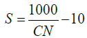 (1)
(1)
CN has a range between 0-100. This relation, which calculates S can then be used to find out the value of Q as:
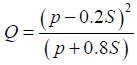 (2)
(2)
Here P is the rainfall in inches. In essence, CN is a parameter that governs the runoff potential, the higher its values, the higher runoff potential is. Considering all the above mentioned probe parameters such as crops stage, time of concentration etc., the aim is to select only the relevant minimum amount of inputs in order to be able to cut the hardware cost by utilizing only the relevant sensors.
The TR 55 is a technical release NRCS detail documentation for urban hydrology for small watersheds, which in this research is used for curve number selection list of scenarios. A total of thirteen different curve numbers have been selected which are 30, 35, 40, 45, 50, 55, 60, 65, 70, 75, 80, 85 and 90 from the Tables 1 and 2 indicated below.
| Cover description | Curve numbers for hydrologic soil group | |||||
|---|---|---|---|---|---|---|
| Cover type | Treatment | Hydrologic condition | A | B | C | D |
| Fallow | Bare soil | -- | 77 | 86 | 91 | 94 |
| Crop residue cover (CR) | Poor | 76 | 85 | 90 | 93 | |
| Good | 74 | 83 | 88 | 90 | ||
| Row crops | Straight row (SR) | Poor | 72 | 81 | 88 | 91 |
| Good | 67 | 78 | 85 | 89 | ||
| SR+CR | Poor | 71 | 80 | 87 | 90 | |
| Good | 64 | 75 | 82 | 85 | ||
| Contoured (C) | Poor | 70 | 79 | 84 | 88 | |
| Good | 65 | 75 | 82 | 86 | ||
| C+CR | Poor | 69 | 78 | 83 | 87 | |
| Good | 64 | 74 | 81 | 85 | ||
| Contoured & terraced (C&T) | Poor | 66 | 74 | 80 | 82 | |
| Good | 62 | 71 | 78 | 81 | ||
| C&T+CR | Poor | 65 | 73 | 79 | 81 | |
| Good | 61 | 70 | 77 | 80 | ||
| Small grain | SR | Poor | 65 | 76 | 77 | 88 |
| Good | 63 | 75 | 84 | 87 | ||
| SR+CR | Poor | 64 | 75 | 83 | 86 | |
| Good | 60 | 72 | 83 | 84 | ||
| C | Poor | 63 | 74 | 80 | 85 | |
| Good | 61 | 73 | 82 | 84 | ||
| C+CR | Poor | 62 | 73 | 81 | 84 | |
| Good | 60 | 72 | 81 | 83 | ||
| C&T | Poor | 61 | 72 | 80 | 82 | |
| Good | 59 | 70 | 79 | 81 | ||
| C&T +CR | Poor | 60 | 71 | 78 | 81 | |
| Good | 58 | 69 | 78 | 80 | ||
| Close seeded or broadcast legumes or rotation meadow | SR | Poor | 66 | 77 | 77 | 89 |
| Good | 58 | 72 | 85 | 85 | ||
| C | Poor | 64 | 75 | 81 | 85 | |
| Good | 55 | 69 | 78 | 83 | ||
| C&T | Poor | 63 | 73 | 80 | 83 | |
| Good | 51 | 67 | 76 | 80 | ||
Table 1: Runoff curve numbers for cultivated agricultural lands.
| Cover description | Curve numbers for hydrologic soil group | ||||
|---|---|---|---|---|---|
| Cover type | Hydrologic condition | A | B | C | D |
| Pasture, grassland, or range-continuous forage for grazing. | Poor | 68 | 79 | 86 | 80 |
| Fair | 49 | 69 | 79 | 84 | |
| Good | 39 | 61 | 74 | 80 | |
| Meadow-continuous grass, protected from grazing and generally mowed for hay. | -- | 30 | 58 | 71 | 78 |
| Brush-brush-weed-grass mixture with brush the major element | Poor | 48 | 67 | 77 | 83 |
| Fair | 35 | 56 | 70 | 77 | |
| Good | 30 | 48 | 65 | 73 | |
| Woods-grass combination (orchard or tree farm) | Poor | 57 | 73 | 82 | 86 |
| Fair | 43 | 65 | 76 | 82 | |
| Good | 32 | 58 | 72 | 79 | |
| Woods | Poor | 45 | 66 | 77 | 83 |
| Fair | 36 | 60 | 73 | 79 | |
| Good | 30 | 55 | 70 | 77 | |
| Farmsteads-buildings, lanes, driveways and surrounding lots | -- | 59 | 74 | 82 | 86 |
Table 2: Runoff curve numbers for other agricultural lands.
Data extraction from NRCS hydrological simulator
Data extraction is done from the NRCS simulator for inputs variables irrigation depth, Curve number, time of concentration and outputs variables Runoff volume. An authenticated database has been generated with random samples from entry number 1 up to entry number 4095. The author has written a detailed script in NRCS simulator to acquire the relevant variables datasets from the NRCS implemented in the Table 3.
| Collected Data | |||||
|---|---|---|---|---|---|
| Depth | CN | TC | Runoff | Runoff Time | |
| 73 | 1 | 75 | 50 | 0.0303 | 26.8889 |
| 74 | 1 | 75 | 80 | 0.0303 | 28.6222 |
| 75 | 1 | 75 | 110 | 0.0303 | 30.3111 |
| 76 | 1 | 75 | 140 | 0.0303 | 32.0444 |
| 77 | 1 | 90 | 50 | 0.3204 | 26.8889 |
| 78 | 1 | 90 | 80 | 0.3204 | 28.6222 |
| 79 | 1 | 90 | 110 | 0.3202 | 30.3111 |
| 80 | 1 | 90 | 140 | 0.3202 | 32.0444 |
Table 3: Shows collected database from the NRCS simulator.
The depth of irrigation is taken in range of 1 up to 15 inches, the curve number values selected within the range of 30 up to 90 on the increment of 5, time of concentration is taken 50 up to 150 minutes with the increment of 5. The NRCS computes and further gives the different numeric values for runoff time unit in hour’s output variable ranges from 1 to 4095 samples.
Experimental Setup
The performance of Machine Learning algorithms is evaluated by different performance metrics using training and testing data set. Given a set of data, only a part of it is typically used to learn a predictive model. This part is referred to as the training set. The remaining part is reserved for evaluating the predictive performance of the learned model and is called the testing set. The testing set is used to estimate the performance of the model on unseen data. More reliable estimates of the performance on unseen data are obtained by using cross validation, which partitions the entire data available into n subsets. Each of these subsets is in turn used as a testing set, with all of the remaining data are used as training set. In this study 2 fold validation, 5 fold validation and 10 fold validation have been used. The performance efficiency of algorithms are also affected by the amount of training data. It is also analyzed that which algorithm show best and worst performance when the amount of training data is in abundance or scarce.
Different data division techniques are used to divide the dataset into training and testing data. These are 70/30 (i.e., 70% data for training and 30% for testing), 30/70 and k-fold techniques.
Case A (30/70): Randomly divided the entire generated data into two subsets. First subset had 30% of the samples generated and it was used to train the regressive models. The second one had remaining 70% of the samples and was used to analyze the authenticity and reliability of the created models by testing. Basic aim here was to gauge if there is any regression model that can yield state of the art results even if it has been trained on very few samples. Training a model on fewer samples guarantees a lower training time of the model. The aim is to deploy such a machine learning algorithm in the network that can give a precise fit on the testing data without having to undergo a lengthy time consuming.
Case B (70/30): In case B experimentation, the aim is to find such an algorithm which gives a near perfect fit on testing data without the need of an extensive training phase.
It is almost similar to the case A scenario, only difference is that here the larger chunk of data (70%) is used to train the system and remaining 30% for testing.
Case C (K fold): In case A and case B, a study is carried out to see the effect of changing ratios of training and testing data on the model evaluation parameters. As a last case, we will study the evaluation results on k- fold validation with k=2, k=5 and k=10. Similarly, after the application of above mentioned machine learning techniques, the results obtained are measured for performance evaluation with different metrics such as Training Time of the samples, Mean Square Error in the results etc.
Evaluation parameters
Every regression model could result in the predicted values being closer to the observed values [32]. For every predicted value, a mean value is used in the mean model, which can be used in the application when there are no informative predictor variables available. As a result, the proposed model fit is better as compared to the fit of the mean model. The RMSE is used as a standard statistical metric to calculate the model performance in climate research studies, meteorology and air quality. The Mean Absolute Error (MAE) also vastly used in model evaluations. There has been no final consensus made on the most appropriate metric for model errors from the two models [33]. In our experimental study we evaluated the four machine learning algorithms i.e., ANN, MLR, DT (Regression) and LS-SVR for runoff volume prediction. For each experiment, we evaluate the results by the following evaluation parameters:
Mean Square Error (MSE): The mean squared error determines how close a set of points is to a regression line. This is done by taking the distances from the set of points to the regression line and squaring them. These distances are the “errors”. The squaring at the end is essential to remove any negative signs and helps give weight to larger differences. It is referred to as the mean squared error as you are evaluating the average of a set of errors [34].
The smaller the value of the MSE, the nearer you are to determining the line of best fit. This depends on the data as well; it might not be possible to get a very small value for the mean squared error. The MSE includes both the variance of the estimator and its bias and is also known as the second moment (about the origin) of the error. MSE is the variance of the estimator for an unbiased estimator. Similar to the variance, MSE uses the same units of measurement as the square of the quantity being estimated [35].
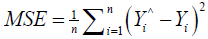 (3)
(3)
Root Mean Square Error (RMSE): The Root Mean Square Error (RMSE) is calculated using the square root of the residuals. It depicts the absolute fit of the model to the data telling how close the observed data points presently are to the model’s predicted values. The R-squared is a relative measure of the fit while RMSE is an absolute measure of the fit. RMSE can also be interpreted as the unexplained variance’s standard deviation, and possesses the property of being in the same units as the response variable. The lower values of RMSE depict a better fit. RMSE is a good measure of how accurately the model predicts the response.
The RMSE with respect to the estimated variable Xmodel is defined as:
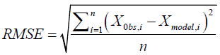 (4)
(4)
Xobs: Observed values
Xmodel: Modelled values at time/place i.
Relative Root Mean Square Error (RRMSE)
The Relative Root Mean Square Error (RRMSE) is denoted by dividing the RMSE by the mean observed data:
RRMSE= RMSE/mean(pred_vals) (5)
Coefficient of determination (R2): R2, is the coefficient of determination [36], which is used to detect how the distinct values in one variable can be used to explain the difference in a second variable [37]. R-squared has a very crucial functionality that its scale is intuitive which means that it ranges from zero to one, with zero illustrating the fact that the proposed model does not improve the prediction over the mean model and one means that it has a perfect prediction. Improvement in the regression model concludes in the proportional rises in R-squared [38].
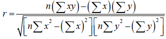 (6)
(6)
Mean Absolute Error (MAE): The Mean Absolute Error (MAE) is the measure of the distinguished values between two continuous variables [39]. It is an average/mean of the absolute error which uses the saw me scale as the data being calculated. It cannot be utilized to make comparisons between series using the different scales [40].
The MAE is the calculation of the forecast error in the time series analysis [41] and is given by:
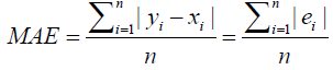 (7)
(7)
Normalized Root Mean Square Error (NRMS): The dimensionless forms of the RMSE are quite handy, as the user often wants to compare RMSE with the distinct units. There are two methods for that:
Normalize the RMSE to the range of the observed data:
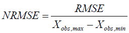 (8)
(8)
Normalize to the mean of the observed data:
 (9)
(9)
Results
Case A results
The Case-A consists of all three inputs, while the training set is taken as 30% random data of the total data set, while 70% of the remaining data is dedicated for the testing purposes. The results are plotted in figures below:
The Case-A (Figures 4-7 and Table 4) shows that with training set of 30% data, except Multiple Linear Regression, all regression algorithms perform well and predict the output efficiently, which in this case is runoff time. Multiple Linear Regression seems to oscillate around the original values. The answer to this lies in the very nature of the MLR: since it is a linear regression model, it is more suitable for the dataset in which the data follows a linear trend; it assumes that there is a straight-line relationship between the dependent and independent variables, which is not the case here. Moreover, consider the average value of dependent variable to predict the output; since average values does not necessarily correspond to the original value of the variable at a given samples, it generates errors.

Figure 4: Input parameters (I, CN, Tc) vs. runoff time output for holdout method 30/70 by ANN.

Figure 5: Input parameters (I, CN, Tc) vs. runoff time output for holdout method 30/70 by MLR.

Figure 6: Input parameters (I, CN, Tc) vs. runoff time output for holdout method 30/70 by SVR.

Figure 7: Input parameters (I, CN, Tc) vs. runoff time output for holdout method 30/70 by DT.
| Training time | MSE | NRMS | R2 | RMSE | RRMSE | MAE | |
|---|---|---|---|---|---|---|---|
| ANN | 0.40866 | 0.0039693 | 0.036437 | 0.99867 | 0.0643003 | 0.0021188 | -0.00041442 |
| MLR | 0.00044302 | 22.644 | 2.7521 | 0.35907 | 4.7586 | 0.16465 | -0.83525 |
| SVR | 47.198 | 0.01749 | 0.076484 | 0.99335 | 0.13225 | 0.0044416 | 0.039149 |
| Decision trees | 0.011535 | 5.8218e-28 | 1.3954e-14 | 1 | 2.4128e-14 | 8.1142e-16 | -6.8155e-15 |
Table 4: Holdout method 30/70 results for input parameters (I, CN, Tc) vs. runoff time output parameter.
The table shows that values of R-squared parameter are close to unity for ANN, SVM and DT. This means that their prediction quality is close to 100% and hence, their mean-squared and meanabsolute errors are close to zero. DT is perfectly 1, i.e., it has predicted all the values correctly using its regression. Second in rank is ANN, whose performance closely resembles that of SVR. However, the training time of SVR is extremely higher than the remaining techniques, which offsets its better prediction capability.
Case B results
Here are the results obtained for 70% of the data samples for training and the remaining 30% for testing. With the increase in training data in Case-B (Figures 8-11 and Table 5), The figures above show that Artificial Neural Networks and Decision Trees both give a good fit on the testing data, Support Vector Machines are not very accurate and Multiple Linear Regression gives worst results. To analyze these two more closely, we look at the table of evaluation parameters, which makes it clear that DT approach is far superior that ANN one- in terms of curve fit on unseen data as well as the training time, since DT gives 100% accuracy because its R-squared parameter is absolute 1 and all the mean-squared (MSE, NRMS, RMSE, RRMSE) and mean absolute errors are close to zero.

Figure 8: Input parameters (I, CN, Tc) vs. runoff time output for holdout method 70/30 by ANN.

Figure 9: Input parameters (I, CN, Tc) vs. runoff time output for holdout method 70/30 by MLR.

Figure 10: Input parameters (I, CN, Tc) vs. runoff time output for holdout 70/30 ratio by SVR.

Figure 11: Input parameters (I, CN, Tc) vs. runoff time output for holdout 70/30 ratio by DT.
Table 5: Holdout method 70/30 results for input parameters (I, CN, Tc) vs. runoff time.
| Training time | MSE | NRMS | R2 | RMSE | RRMSE | MAE | |
|---|---|---|---|---|---|---|---|
| ANN | 1.1536 | 0.0037227 | 0.035615 | 0.99873 | 0.061014 | 0.0020518 | -0.00089898 |
| MLR | 0.034359 | 22.429 | 2.7645 | 0.3545 | 4.7359 | 0.16511 | -1.0541 |
| SVR | 120.46 | 0.015556 | 0.072805 | 0.99403 | 0.12472 | 0.0041889 | 0.038056 |
| Decision trees | 0.25618 | 1.165e-26 | 6.3004e-14 | 1 | 1.0793e-13 | 3.6296e-15 | -8.7922e-14 |
Case C results
Case-C (Figures 12-15 and Tables 6-8) comprises identical regression algorithm as done in previous cases, except that the division of dataset for training and testing is done in a new fashion. Three experiments were performed using k-fold distribution, that is, dividing the dataset into k subsets and then using some subsets for training and other for testing. This generates k different results, which can be merged into one result by taking their mean, for each value of k. The results attained are listed in the table below, while figures show the visual content only for fold 5 of k=5, K=2, K=5.

Figure 12: ANN performance for fivefold cross validation.

Figure 13: MLR performance for fivefold cross validation.

Figure 14: SVR performance for fivefold cross validation.

Figure 15: DT performance for fivefold cross validation.
Table 6: Twofold cross validation result.
| Training time | MSE | NRMS | R2 | RMSE | RRMSE | MAE | |
|---|---|---|---|---|---|---|---|
| ANN | 1.0159 | 0.0037723 | 0.035461 | 0.00874 | 0.061416 | 0.0020659 | 0.001577 |
| MLR | 0.00062754 | 22.514 | 2.7396 | 0.36265 | 4.7448 | 0.16481 | -0.93676 |
| SVR | 0.15821 | 0.015757 | 0.69699 | 0.99409 | 0.12553 | 0.0042172 | 0.038768 |
| Decision trees | 0.061167 | 2.0274e-27 | 2.5652e-14 | 1 | 4.4429e-14 | 1.4946e-15 | -2.9487e-14 |
Table 7: Fivefold cross validation results.
| Training time | MSE | NRMS | R2 | RMSE | RRMSE | MAE | |
|---|---|---|---|---|---|---|---|
| ANN | 2.0547 | 0.0032507 | 0.032789 | 0.99891 | 0.056809 | 0.0019111 | -0.0012473 |
| MLR | 0.0004821 | 22.531 | 2.739 | 0.36291 | 4.7456 | 0.16484 | -0.93733 |
| SVR | 0.10789 | 0.015757 | 0.96761 | 0.99409 | 0.12553 | 0.0042172 | 0.038769 |
| Decision trees | 0.018101 | 6.3157e-27 | 4.5869e-14 | 1 | 7.9471e-14 | 2.6734e-15 | 4.8046e-14 |
Table 8: Tenfold cross validation method input parameters (I, CN, Tc) vs. runoff time output parameter.
| Training time | MSE | NRMS | R2 | RMSE | RRMSE | MAE | |
|---|---|---|---|---|---|---|---|
| ANN | 4.7841 | 0.00012743 | 0.0030131 | 0.9999 | 0.010712 | 0.0028244 | 4.2904e-05 |
| MLR | 0.00098281 | 3.357 | 0.51423 | 0.52195 | 1.8316 | 0.44753 | 0.2894 |
| SVR | 0.94477 | 1.2772 | 0.62925 | 0.90181 | 1.1276 | 0.30706 | -0.12812 |
| Decision trees | 0.01831 | 3.2202e-05 | 0.0015836 | 1 | 0.0056398 | 0.0014837 | 0.00010243 |
The k=5 fold cross validation graphs are as follow:
In all three cases of k, decision tree dominates the regressive schemes with its close to 100% accuracy, minimum (or even negligible) mean-squared (MSE, NRMS, RMSE, RRMSE) and Mean Absolute Errors (MAE) and lower training time. In fact, its training time is lowest after MLR. But since MLR has shown worst performance in all scenarios, it cannot be used practically in these cases. The reason is already cited, that MLR is appropriate for datasets, which follow linear or close to linear relationship. The second best performance is by ANN in terms of error reduction; however, its training time is higher as compared to DT and SVR.
The SVR shows intermediate performance in terms of its accuracy, however, its training time is much lesser than ANN’s.
From the analysis of three cases: case A, case B and case C, it can be concluded that SVR performs better in terms of training time when used with cross-validation. The training time of SVR rises sharply in case of data division into two parts as in cases A and B. This problem resides in the kernel of SVR, which needs huge amount of memory as well as contributes to the complexity of this algorithm. SVR computes the distance function between each point of the dataset, which makes the computations lengthier.
In all the cases of this chapter, ANN and DT have been efficient in minimizing the error, but as mentioned many times before, DT dominates the overall results owing to its minimum training time, while ANN’s training time is comparatively higher. Thus, Decision Tree can be regarded as the best algorithm for regression.
Discussion and Conclusion
From the previous research, it is worth to be noticed that machine learning algorithms have been deployed in variety of hydrological problems such as flood forecasting, stream or river forecasting, dam or water reservoir level forecasting, rainfall-runoff predication and an irrigation runoff/decision support modelling, however from the machine learning context the algorithms that have been widely used previously are MLR, ANN, SVM in these hydrological and agriculture domains which have their pros and cons. Now from the current research perspective decision trees particularly regression tree and model trees (M5 tree) have been used in these areas which has shown some phenomenal results as compare to MLR, ANN and SVM, however the work done on model trees is very limited so far and is very novel that has been explored in the hydro agricultural domain. The pros over ANN is decision tree, regression tree and model tree (M5 tree) are transparent, easy to understand, fast to train, easily converge and good accuracy. The best algorithm to be used in machine learning and deployed on the sensor networks node depends on different factors and requirements including performance, computation cost, memory requirement and ease of use etc. Moreover, the constraints of limited battery power stipulates that algorithm to be used should consume minimum battery power and avoids an extended training process. MLR is the simplest of all learning methods and requires minimum training time and computation power. However, its performance is very low in cases of non-linear problems. Hence, the use of MLR in non-linear problems is very limited and usually out of question. MLR worse performance is also reflected in the above results having (R-square of around 0.5 and higher MSE value in all the cases a-c) that has been generated for the predication of runoff time as compare to all the other algorithms used. The least square support vector regression is used in this work has shown intermediate results in terms of R-square around 0.994, second highest MSE value after MLR and second highest training time required after ANN in case a and case b, however in terms of case c (k=2, k=5, k=10 fold- cross validation) its training time decreases sharply. The most common model of ANN uses back-propagation for training purposes, containing at least one hidden layer along with one input and output layer. However, in this work, ANN (levenberg-Marquardtt back propagation) has been used and the hidden layer contains of 10 neurons. ANN is an efficient and widely used algorithm which works well with the training and testing of all the cases a, b and c as its R-square is around 0.998 while its MSE is lesser than MLR, LS-SVR and only higher than regression tree, its training time is very much faster in case a and case b than LS-SVR however in case c (different k fold cross validation) the LSSVR training time slightly improves. Thus, in overall comparison MLR and LS-SVR, the ANN (LMA) performs well however its showcased slightly degraded performance in terms of training time, MSE, RMSE, NRMSE, MAE and R-square when compared with regression tree. The conclusive remarks are depicted from above graphs and tables generated from NRCS hydrological simulator in MATLAB tool that Decision tree (regression tree) perform very outstanding in this dataset collected, For case a, b and c regression tree showed outstanding performance of perfect r-square value=1 and minimum MSE=0, RMSE=0, NRMS=0, MAE=0. Thus decision tree (regression tree) place first ranked and an ideal algorithm to be deployed on the sensor node keeping in view all the constraints of the sensor node for the runoff time predication.
REFERENCES
- UNEP FI, SIWI Challenges of water scarcity: A business case for financial institutions. The United Nations Environment Programme Finance Initiative (UNEP FI). 2004.
- Bernstein S. Freshwater and human population: A global perspective. Yale School of Forestry and Environmental Studies Bulletin. 2002;pp:149-157.
- Tanji KK, Kielen NC. Agricultural drainage water management in arid and semi-arid areas. Rome: FAO. 2002.
- Winpenny J, Heinz I, Koo-Oshima S. The wealth of waste: The economics of wastewater use in agriculture. Food and Agriculture Organization of The United Nations, Rome (Italy). 2010.
- Moss B. Water pollution by agriculture. Philos Trans R Soc Lond B Biol Sci. 2008;363:659-666.
- U EPA. National water quality inventory: Report to Congress. Washington, DC. 2009.
- Water UN. Coping with water scarcity: A strategic issue and priority for system-wide action. UN-Water: Geneva, Switzerland. 2006.
- Marks G. Precision irrigation: a method to save water and energy while increasing crop yield, a targeted approach for California Agriculture. 2010.
- Patil P. Intelligent irrigation control system by employing wireless sensor networks. IJCA. 2013;79:33-40.
- Goumopoulos C, O’Flynn B, Kameas A. Automated zone-specific irrigation with wireless sensor/actuator network and adaptable decision support. Comput Electron Agr. 2014;105:20-33.
- Mohapatra A, Kumar SL. Neural network pattern classification and weather dependent fuzzy logic model for irrigation control in WSN based precision agriculture. Procedia Computer Sci. 2016;78:499-506.
- Zhang M, Li M, Wang W, Liu C, Gao H. Temporal and spatial variability of soil moisture based on WSN. Math Comput Model. 2013;58:826-833.
- Navarro-Hellín H, Martínez-del-Rincon J, Domingo R, Valles-soto F, Torres R. A decision support system for managing irrigation in agriculture. Comput Electron Agr. 2016;125:121-131.
- Wan S. Research on the model for crop water requirements in wireless sensor networks. Management of e-Commerce and e-Government (ICMeCG), 2012 International Conference on, Beijing, P.R. China. 2012.
- http://www.professorpatel.com/curve-number-introduction.html
- Wilby RL, Abrahart RJ, Dawson CW. Detection of conceptual model rainfall-runoff processes inside an artificial neural network. HSJ. 2003;48:163-181.
- Rasouli K, Hsieh WW, Cannon. A Daily streamflow forecasting by machine learning methods with weather and climate inputs. J Hydrol. 2012;414:284-293.
- Kuzmanovski V. Integration of expert knowledge and predictive learning: Modelling water flows in agriculture. Jofief Stefan International Postgraduate School, Ljubljana, Slovenia. 2012;pp:1-138.
- Ishak WHW. Neural network application in reservoir water level forecasting and release decision. IJNCAA. 2011;pp:265-274.
- Botsis D, Latinopoulos P, Diamantaras K. Rainfall-runoff modeling using support vector regression and artificial neural networks. 12th International Conference on Environmental Science and Technology (CEST2011), Rhodes, Greece. 2011.
- Zakaria ZA, Ani S. Streamflow forecasting at ungaged sites using support vector machines. Appl Math Sci. 2012;6:3003-3014.
- Gill MK, Asefa T, Kemblowsk MW, McKee M. Soil moisture prediction using support vector machines. JAWRA. 2006;pp:1033-1046.
- Wu W, Wang X, Xie D, Liu H. Soil water content forecasting by support vector machine in purple hilly region. CCTA. 2007;1:223-230.
- Ahmad S, Stephen H, Kalra A. Estimating soil moisture using remote sensing data: A machine learning approach. Adv Water Resour. 2010;33:69-80.
- Zia H, Harris N, Merrett VG. Water quality monitoring, control and management (WQMCM) framework using collaborative wireless sensor networks. 11th International Conference on Hydroinformatics (HIC), United States, New York. 2014.
- Khan SA, See LM. Rainfall-runoff modelling using data driven and statistical methods. Advances in Space Technologies, 2006 International Conference, Islamabad. 2006.
- Solomatine PD, Dulal NK. Model trees as an alternative to neural networks in rainfall-runoff modelling. Hydrolog Sci J. 2003;48:399- 411.
- Solomatine PD, Xue Y. M5 model trees and neural networks: Application to flood forecasting in the upper reach of the Huai River in China. J Hydrol Eng. 2004;9:491-501.
- Kuzmanovski V, Trajanov A, Leprince F, Dzeroski S, Debeljak M. Modelling water outflow from tile-drained agricultural fields. Sci Total Environ 2015;505:390-401.
- Khan M, Noor S. Irrigation runoff volume prediction using machine learning algorithms. EIJST. 2019;8:1-22.
- Cronshey R. TR-55: Urban hydrology for small watersheds. United States Department of Agriculture. 1986;pp:1-164.
- http://www.theanalysisfactor.com/
- Chai T, Draxler RR. Root mean square error (RMSE) or mean absolute error (MAE)?- Arguments against avoiding RMSE in the literature. GMD. 2014;7:1247-1250.
- http://www.statisticshowto.com/mean-squared-error/
- https://en.wikipedia.org/wiki/Mean_squared_error
- Dufour JM. Coefficients of determination. McGill University. 2011;pp:1-14.
- http://www.statisticshowto.com/what-is-a-coefficient-ofdetermination/
- Ohtani K, Tanizaki H. Exact distributions of R2 and distributed R2 in a linear regression model with multivariate error terms. J Japan Statist SOC. 2004;34:101-109.
- Willmott CJ, Kenji M. Advantages of the mean absolute error (MAE) over the root mean square error (RMSE) in assessing average model performance. Clim Res. 2005;30:79.
- https://otexts.com/fpp2/accuracy.html
- Hyndman JR, Koehler BA. Another look at measures of forecast accuracy. Int J Forecasting. 2005;22:679-688.
Citation: Khan M, Noor S (2019) Performance Analysis of Regression-Machine Learning Algorithms for Predication of Runoff Time. Agrotechnology 8:187. doi: 10.35248/2168-9881.19.8.187
Copyright: © 2019 Khan M, et al. This is an open-access article distributed under the terms of the Creative Commons Attribution License, which permits unrestricted use, distribution, and reproduction in any medium, provided the original author and source are credited.