PMC/PubMed Indexed Articles


Indexed In
- Academic Journals Database
- Open J Gate
- Genamics JournalSeek
- Academic Keys
- JournalTOCs
- China National Knowledge Infrastructure (CNKI)
- CiteFactor
- Scimago
- Ulrich's Periodicals Directory
- Electronic Journals Library
- RefSeek
- Hamdard University
- EBSCO A-Z
- OCLC- WorldCat
- SWB online catalog
- Virtual Library of Biology (vifabio)
- Publons
- MIAR
- University Grants Commission
- Geneva Foundation for Medical Education and Research
- Euro Pub
- Google Scholar
Useful Links
Share This Page
Journal Flyer

Open Access Journals
- Agri and Aquaculture
- Biochemistry
- Bioinformatics & Systems Biology
- Business & Management
- Chemistry
- Clinical Sciences
- Engineering
- Food & Nutrition
- General Science
- Genetics & Molecular Biology
- Immunology & Microbiology
- Medical Sciences
- Neuroscience & Psychology
- Nursing & Health Care
- Pharmaceutical Sciences
Research - (2020) Volume 12, Issue 6
Non-linear Mixed Effects Modeling and Simulation for Exploring Variability Sources in Dissolution Curves: A BCS Class II Case Example
Eleni Karatza1,2* and Vangelis Karalis1,22Institute of Applied and Computational Mathematics (IACM)/Foundation of Research and Technology Hellas (FORTH), Greece
Received: 30-Sep-2020 Published: 30-Nov-2020, DOI: 10.35248/0975-0851.20.12.406
Abstract
Purpose: Irbesartan is a BCS class II compound that exhibits pH– and buffer capacity–dependent dissolution behavior. The aim of this study was to apply non-linear mixed effects modelling on dissolution data of two immediate release products containing Irbesartan in order to characterize and quantify the sources of inter-dissolution profile variability.
Methods: Nonlinear mixed effects modelling was applied to describe the dissolution curves obtained for Irbesartan in three different pH-value media (1.2, 4.5, 6.8) with two different products (reference product: Aprovel® and a generic test product). Simulations performed and the impact of inter-dissolution variability was assessed.
Results: The % Irbesartan dissolved to time was found to follow a Weibull distribution. Τhe population scale parameter was estimated 0.252 and the shape parameter was estimated 0.706. The pH-value of the dissolution medium was found to significantly affect the scale parameter, while the formulation was found to affect the shape parameter. Simulations showed that probably some discrepancies in the in vivo performance of the two products can be expected.
Conclusion: Through this case study the applicability and usefulness of nonlinear mixed effects modelling in oral drug formulation was highlighted and resides in its ability to identify and quantify sources of variability.
Keywords
Population modeling; Simulations; Dissolution; Irbesartan; BCS Class II
Introduction
Irbesartan is highly permeable but presents low aqueous solubility and thus belongs to BCS class II compounds. It has been claimed to present both weak acidic and weak basic properties [1-4]. In view of the complex environment of the gastrointestinal tract (GI) involving pH gradient and variation in the buffer capacity and ionic strength of GI fluids, BCS class II compounds present significantly different dissolution profile within each GI region [4,5]. As a result, dissolution studies in various pH media are highly informative of the expected in vivo performance [2,6], while some in vitro transfer models simulating the conditions and the residence time in within each region of the GI tract have also been proposed [5].
In vitro dissolution testing is a very important tool for drug development and quality control, as well as for investigation of bioequivalence [7-10]. Application of pharmacometrics, i.e., the quantitative evaluation and mathematical description of the in vitro dissolution experiments, may offer significant insight regarding the underlying processes that take place, their kinetics and the sources of variability [11,12]. The main sources of variability in dissolution testing have been reported to be the analyst, the dissolution apparatus, the testing environment, the sample and naturally the product under investigation [8,9]. Various equations and mathematical approaches have been applied in order to characterize and study the dissolution profiles retrieved from in vitro dissolution studies either for research or for regulatory purposes [8,9,11,13-15]. Even a computer program has been developed that provides a model library for fitting dissolution data and facilitates the comparison of drug dissolution data [8].
However, in the case where the there is a need to study, quantify and understand the sources of variability, nonlinear mixed effects modeling (nlme) is the more appropriate mathematical approach. Nlme consists of the identification of a model for the typical response (structural model), a model for heterogeneity which involves the predictable and unexplained reasons responsible for inter-individual variability and a model for uncertainty (residual error model) which describes why the previous two models do not much our observations exactly [16]. This technique has been applied, in a previous study with the aim to assess its contribution in the comparison of dissolution curves obtained for several batches of sustained release formulations of octreotide [13]. However, up to now it has not been applied clearly for the study of variability among dissolution curves.
The aim of the present study was to apply non-linear mixed effects modeling on dissolution data retrieved from two different products containing 300 mg of Irbesartan in order to describe its dissolution curves and quantify the impact of medium’s pH and formulation on them. Secondarily through this case study, the present work aims to highlight the advantages that nonlinear mixed effects modeling and simulation may offer in oral drug development.
Methodology
Dissolution data
Dissolution data were retrieved from tests designed for the in vitro comparison of pilot batches of a generic film coated tablet formulation containing 300 mg of Irbesartan with the reference product Aprovel® 300 mg. A dissolution USP II paddle apparatus was used, while the experiments were performed in three different mediums with pH values 1.2, 4.5 and 6.8. The dissolution experiments were performed in accordance to the EMA guideline on the investigation of bioequivalence [7]. Samples were collected at pre-defined time points and the % amount dissolved was calculated. In view of the fact that Irbesartan presents a pHdependent dissolution behavior [1] a different sampling scheme was applied for studying the dissolution kinetics in each medium. Each experiment was replicated 12 times; as a result data from a total of 72 dissolution experiments were retrieved. Each dissolution experiment was considered as a separate individual, in order to perform a population analysis.
Nonlinear mixed effects modelling
Monolix Suite® 2019R2 (Lixoft, Orsay France) was used as software in order to apply non-linear mixed effects modeling. All model parameters were assumed to follow a lognormal distribution, and an exponential model was used to describe inter individual variability.
Structural model
The initial dose was set at 100, as the % dissolved was used as dependent variable and a nonlinear mixed effect model was seeked for % dissolved (t). The models explored were the simple first order with only one parameter standing for a first order dissolution rate constant (kd), the Weibull model with a scale and shape parameter, Korsmeyer-Peppas (Power Law) with a kinetic constant and an exponent characterizing the diffusion mechanism and the logistic function with a scale, a shape and a location parameter. These models were selected as they are models that have been found to efficiently describe dissolution kinetics [8,9,14,15].
Modeling inter-individual and residual variability
The impact of formulation type (reference or test) and pH value of the medium (1.2, 4.5 or 6.8) were explored as potential categorical covariates on model parameters. Statistical significance of these categorical was assessed by a one-way ANOVA. A Wald test and a Likelihood ratio test (LRT) were used in order to decide their inclusion in the model. A significance level of 5% was considered in all cases. Different error models of residual variability (constant, proportional, combined) were assessed based on the OFV but also on the model evaluation and validation criteria as analyzed below.
Model evaluation and validation
The models were evaluated both graphically (goodness of fit plots) and statistically (-2LL, Akaike and Bayesian information criteria). More specifically the goodness of fit plots inspected were primarily the individual fittings of the predicted profile given by the estimated individual model versus the observed data and the population and individual predictions overlaid on observations versus time. The predictive performance was assessed by prediction corrected visual predictive checks (VPCs) generated using Monte Carlo simulations of 1,000 datasets and 90% prediction intervals.
Simulations
Simulations were performed the expected range of dissolution profiles based on the estimated variability and have a more robust assessment of the dissolution behavior. Taking into account the inter-dissolution variability, a total of 500 dissolution profiles were simulated in each case and the effect of pH and formulation on the dissolution curves was explored more in depth without the need to perform any additional experiments.
The R function ‘Simulx’ included in the ‘mlxR’ package was used to perform the simulations.
Results and Discussion
All dissolution data included in this analysis are presented in Figure 1. A population model able to describe the dissolution profiles of Irbesartan was successfully developed. A Weibull model was found to most adequately fit the data. The parameters estimated for the model are presented in Table 1. The accuracy and reliability of the parameter estimates obtained, was confirmed by the low % RSE values. The model described the data adequately as shown by the individual fittings of the predicted profile given by the estimated individual model versus the observed data (Figure 2) and by the individual predictions overlaid on observations (Figure 3A). The robustness and predictive capacity of the model can be noted by the VPC and the observed versus predicted plot (Figure 3B).

Figure 1: Spaghetti plot of the observed dissolution profiles per formulation and per pH of the medium used for the experiment. Therefore yellow represents the dissolution profiles retrieved with the reference product in a medium of 1.2 pH value, red with the test product in a medium of 1.2 pH value, pink with the reference product in a medium of 4.5 pH value, orange the test product in a medium of 4.5 pH value, blue with the reference product in a medium of 6.8 pH value and black with the test product in a medium of 6.8 pH value.

Figure 2: Fittings of the predicted profile given by the estimated individual model versus the observed data. The purple line represents the individual predicted profiles and the black closed circles the observed data.

Figure 3: Goodness of fit plots of the final model developed for the % amount of irbesartan dissolved. On the left: Individual predictions overlaid on observations, On the right: Prediction corrected visual predictive check (VPC) of the Weibull model developed using 1000 Monte Carlo simulations. Median (solid line), 10th, 50th and 90th percentiles (blue line) of the observed data overlaid to the 90 % confidence intervals (colored areas) for the median, 10th, 50th and 90th percentiles of the simulated data.
The Weibull model even though is an empirical equation, it can be applied to almost all kinds of dissolution curves [14]. It expresses the % cumulative amount dissolved to time by:
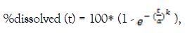
Where a, the scale parameter that defines the time scale of the process and k the shape parameter that characterizes the curve as either exponential (k=1), sigmoid (k>1) or parabolic (k<1) [14]. In the model developed in this study the pH value of the medium was found to significantly affect the scale parameter as described below:
a = a_pop × exp (-0.268)cat1 × exp (-0.773)cat2 × exp (ηa)
Where a_pop equals to the population parameter estimate, ηa represents the random effect, cat1 takes the value 1 when the medium has pH=4.5 and cat2 takes the value 1 when the medium has pH=6.8, otherwise they take the value 0. Evidently, the scale parameter equals to 0.252* exp (ηa), 0.192* exp (ηa) and 0.116* exp (ηa) for a pH medium of 1.2, 4.5 and 6.8, respectively. These findings are in line with the pH-dependent dissolution behavior of Irbesartan [1-4]. Also, it is evident from the faster dissolution rate, i.e., higher time scale parameter that Irbesartan’s basic properties prevail in aqueous media [3].
The formulation type was found to significantly affect the shape parameter as described below:
k = k_pop × exp (-0.134)cat × exp (ηk)
Where k_pop equals to the population parameter estimate, ηk represents the random effect, cat takes the value 1 for the test formulation and 0 for the reference formulation. Therefore, for the reference product the shape parameter equals to 0.706* exp (ηk) and for the test product to 0. 617* exp (ηk). This finding indicates that the curves present the same shape as expected.
A statistically significant inverse correlation between the random effects of the shape and scale parameter was also identified (Table 1), indicating that probably when the one grows the other lessens. This fact may lead to the assumptions that from a kinetic point of view there are some restrictions regarding the shape of the curve in relation to the time scale of the phenomenon.
Table 1: Population estimates identified for the description of irbesartan’s dissolution kinetics following a Weibull distribution.
| Fixed effects | ||||
|---|---|---|---|---|
| Variables | Estimate | SE | RSE (%) | p-value |
| a_pop | 0.252 | 0.0111 | 4.41 | -- |
| beta_PH_45 | -0.268 | 0.0273 | 10.2 | 0.00001 |
| beta_PH_68 | -0.773 | 0.0286 | 3.71 | -- |
| k_pop | 0.706 | 0.017 | 2.41 | -- |
| beta_Formulation_Test | -0.134 | 0.0125 | 9.34 | 0.00175 |
| Standard deviation of the random effects | ||||
| Variables | Estimate | SE | RSE (%) | -------- |
| omega_a | 0.344 | 0.0296 | 8.62 | |
| omega_k | 0.194 | 0.0167 | 8.6 | |
| Correlations | ||||
| Variables | Pearson correlation coefficient | SE | RSE (%) | |
| corr_k_a | -0.964 | 0.00861 | 0.893 | |
| Variables | Proportional error model parameters | SE | RSE (%) | |
| Prop. (%) | 1.80% | 0.000826 | 4.4 | |
Even though the Weibull model effectively characterized the dissolution profiles retrieved, this model doesn’t include any kinetic fundament able to characterize the dissolution kinetic properties of the drug [14-16]. However, the combination of this equation to fit the data and nonlinear mixed effects modeling that is able to identify and quantify the sources of inter-profile variability, the effect of the formulation and the pH medium on the dissolution profiles were quantified.
Through simulations, it was noted that in all three pH the reference formulation presented a rather faster dissolution rate than the test formulation (Figure 4), indicating that probably in vivo some discrepancies of product performance should be expected. In addition, profiles obtained in media with higher pH values present a significantly higher variability, probably because Irbesartan’s dissolution in acidic pH is faster. The significant impact of pH on dissolution of Irbesartan was noted both in simulated profiles of the reference and of the test product. Profiles obtained in media with pH 6.8 showed a much slower solubility than in pH 1.2 confirming the pH-dependent dissolution behavior of the compound and its basic properties.

Figure 4: Simulated dissolution profiles (n=500) in three pH media, namely 1.2, 4.5 and 6.8. Red lines indicate profiles expected with the reference product (Aprovel®) and blue lines with the test product.
Conclusions and Future Work
Nonlinear mixed effects modeling and simulation help to gain a deeper understanding of the dissolution process as well as how various factors impact the dissolution curves. In the case example presented herein the impact of pH and formulation on dissolution curves of Irbesartan (BCS class II) were addressed. In fact, using these techniques, it was noted that due to inter-dissolution variability some differences in the in vivo dissolution and by extension in vivo absorption should be expected. In this vein, it would be interesting to explore the impact of various excipients and/or their percentage in the formulation on dissolution kinetics. Nonlinear mixed effects modeling may constitute a valuable tool for formulation development that could provide guidance to the R&D department for formulation optimization.
Acknowledgements
The authors wish to thank Elpen Pharmaceuticals for providing the dissolution data.
Funding
No funding was received.
Conflicts of Interest/Competing Interests
The authors declare that they have no conflict of interest.
Availability of Data and Materials
The data may be available upon request, even though that can be easily retrieved from Figure 1.
Code Availability
Monolix Suite® 2019R2 (Lixoft, Orsay France) was used.
Authors' Contributions
E.K. performed the modeling exercise, the simulations and contributed to the writing and editing of the manuscript. V.K. conceptualized the study, supervised the computational work and contributed to the writing and editing of the manuscript.
REFERENCES
- Sjögren E, Westergren J, Grant I, Hanisch G, Lindfors L, Lennernäs H, et al. In silico predictions of gastrointestinal drug absorption in pharmaceutical product development: application of the mechanistic absorption model GI-Sim. Eur J Pharm Sci. 2013;49(4):679-698.
- Tsume Y, Mudie DM, Langguth P, Amidon GE, Amidon GL. The Biopharmaceutics Classification System: subclasses for in vivo predictive dissolution (IPD) methodology and IVIVC. Eur J Pharm Sci. 2014;57:152-163.
- Kaur N, Thakur PS, Shete G, Gangwal R, Sangamwar AT, Bansal AK. Understanding the Oral Absorption of Irbesartan Using Biorelevant Dissolution Testing and PBPK Modeling. AAPS PharmSciTech. 2020;21(3):102.
- Hamed R. Physiological parameters of the gastrointestinal fluid impact the dissolution behavior of the BCS class IIa drug valsartan. Pharm Dev Technol. 2018;23(10):1168-1176.
- Hamed R, Kamal A. Concentration Profiles of Carvedilol: A Comparison Between in vitro Transfer Model and Dissolution Testing. J Pharm Innov. 2019;14:123-131.
- Tsume Y, Langguth P, Garcia-Arieta A, Amidon GL. In silico prediction of drug dissolution and absorption with variation in intestinal pH for BCS class II weak acid drugs: ibuprofen and ketoprofen. Biopharm Drug Dispos. 2012;33(7):366-77.
- European Medicines Agency (EMA) Committee For Medicinal Products For Human Use (CHMP), Guideline On The Investigation Of Bioequivalence, Doc. Ref.: CPMP/EWP/QWP/1401/98 Rev. 1/ Corr **, London, UK (2010).
- Zhang Y, Huo M, Zhou J, Zou A, Li W, Yao C, et al. DDSolver: an add-in program for modeling and comparison of drug dissolution profiles. AAPS J. 2010;12(3):263-271.
- Gao P, Shi Y. Characterization of super-saturatable formulations for improved absorption of poorly soluble drugs. AAPS J. 2012;14(4):703-713.
- Shrivas M, Khunt D, Shrivas M, Choudhari M, Rathod R, Misra M. Advances in In vvo Predictive Dissolution Testing of Solid Oral Formulations: How Closer to In vivo Performance?. J Pharm Innov. 2019;15:296-317.
- Marroum PJ. Development, Evaluation, and applications of in vitro/in vivo correlations: A regulatory perspective, Chapter 46 in Pharmacometrics: The Science of Quantitative Pharmacology Edited by Ene I. Ette and Paul J. Williams, John Wiley & Sons, Inc. Hoboken, New Jersey. 2007;pp:1157-1174.
- Williams PJ, Ette EI. Pharmacometrics: Impacting Drug Development and Pharmacotherapy. Chapter 1 in Pharmacometrics: The Science of Quantitative Pharmacology Edited by Ene I. Ette and Paul J. Williams, John Wiley & Sons, Inc. Hoboken, New Jersey, USA. 2007;pp:1-24.
- Comets E, Mentré F. Evaluation of tests based on individual versus population modeling to compare dissolution curves. J Biopharm Stat. 2001;11(3):107-123.
- Costa P, Sousa Lobo JM. Modeling and comparison of dissolution profiles. Eur J Pharm Sci. 2001;13(2):123-133.
- Gao Z. Mathematical modeling of variables involved in dissolution testing. J Pharm Sci. 2011;100(11):4934-4942.
- Duffull SB, Wright DF, Winter HR. Interpreting population pharmacokinetic-pharmacodynamic analyses - A clinical viewpoint. Br J Clin Pharmacol. 2011;71(6):807-814.
Citation: Karatza E, Karalis V (2020) Non-linear Mixed Effects Modeling and Simulation for Exploring Variability Sources in Dissolution Curves: A BCS Class II Case Example. J Bioequiv Availab. 12:406. doi: 10.35248/0975-0851.20.12.406.
Copyright: © 2020 Karatza E, et al. This is an open-access article distributed under the terms of the Creative Commons Attribution License, which permits unrestricted use, distribution, and reproduction in any medium, provided the original author and source are credited.