Indexed In
- Open J Gate
- Genamics JournalSeek
- ResearchBible
- RefSeek
- Directory of Research Journal Indexing (DRJI)
- Hamdard University
- EBSCO A-Z
- OCLC- WorldCat
- Scholarsteer
- Publons
- MIAR
- Euro Pub
- Google Scholar
Useful Links
Share This Page
Journal Flyer

Open Access Journals
- Agri and Aquaculture
- Biochemistry
- Bioinformatics & Systems Biology
- Business & Management
- Chemistry
- Clinical Sciences
- Engineering
- Food & Nutrition
- General Science
- Genetics & Molecular Biology
- Immunology & Microbiology
- Medical Sciences
- Neuroscience & Psychology
- Nursing & Health Care
- Pharmaceutical Sciences
Research Article - (2019) Volume 8, Issue 1
A Generic Workflow for Bioprocess Analytical Data: Screening Alignment Techniques and Analyzing their Effects on Multivariate Modeling
Rajamanickam V1*, Herwig C2 and Spadiut O12Christian Doppler Laboratory for Mechanistic and Physiological Methods for Improved Bioprocesses, Institute of Chemical, Environmental and Biological , TU Wien, Vienna, Austria
Received: 03-Dec-2018 Published: 02-Jan-2019, DOI: 10.35248/2161-1009.19.8.373
Abstract
UV chromatographic data in combination with multivariate data analysis (MVDA) has been extensively used for bioprocess monitoring. However, they are usually attributed to shifts along the retention time and require preprocessing. Misaligned UV chromatographic data result in inconsistent MVDA models. Numerous preprocessing techniques are available, each varying in the number of meta-parameters to optimize, complexity and computational time. Therefore, we aimed at developing a generic workflow to screen for preprocessing techniques. We chose four datasets with increasing complexity containing UV chromatographic data from reverse-phase and size exclusion chromatography HPLC. We aligned all four datasets using three preprocessing techniques, namely icoshift, PAFFT and RAFFT algorithms. We chose several statistical tools to validate the performance of the preprocessing techniques and to screen for meta-parameters. We validated the performance of the preprocessing techniques in terms of data preservation, complexity and computational time, and identified the optimal ranges of meta-parameters for each dataset. Finally, we established principal component analysis (PCA) models to evaluate the chosen alignment technique. Summarizing, in this study a generic workflow has been developed to validate alignment of chromatographic data using statistical tools.
Keywords
Preprocessing; Fingerprinting; Ultraviolet; HPLC; Alignment; CorrectionIntroduction
UV chromatography is a powerful tool, extensively used in bioprocess analytical techniques for quantitative and qualitative analysis [1,2]. The main advantages of UV chromatography are short analysis time, ability to generate high amounts of data containing process information, wide variety of column chemistry and high precision. However, UV chromatographic data are prone to shifts along the retention time, which render subsequent automation and establishment of modeling techniques cumbersome or even impossible. Particularly in biochemical assays done with label free LC analysis, alignment of various analyte profiles to their respective retention time would be of utmost importance [3,4]. HPLC is often coupled with different techniques for biochemical analysis [5-7]. Automation of such assays for extracting valuable process information in bioprocesses for real time analysis would necessitate correcting misalignments in peak profiles. In the past decades, various alignment techniques have been used to correct shifts along the retention time. Peak alignment is necessary for peak identification and quantification, but more importantly for automation and application of subsequent chemometric models, such as principal component analysis (PCA), hierarchical cluster analysis (HCA) and partial lease squares (PLS). For establishing such multivariate models, the chromatographic dataset must contain information about the changes in the process, which are associated with changes in the UV chromatograms. In other words, the retention time of a particular compound must not vary across different samples, as otherwise the predictive ability of the model is compromised [8,9]. A typical UV chromatogram with retention time shifts is shown in Figure 1.
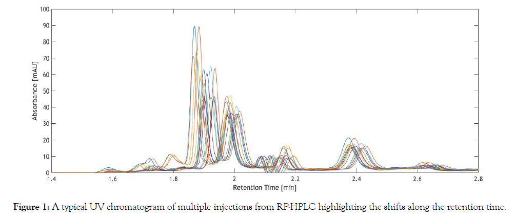
Figure 1: Challenges and requirements of peak alignment techniques.
Various peak alignment approaches to correct misalignments in retention time have been proposed in literature. Most alignment techniques require a reference chromatogram and additional metaparameters for misalignment correction. These meta-parameters are dependent on the dataset and have to be screened in a case-by-case approach [10]. Various target functions for alignment are also used, with the most common being Pearson correlation coefficient [11], Euclidean distance [12], fast Fourier transform (FFT) cross correlation [13] and other even more sophisticated methods. In general, the peak alignment techniques have three different correction methods, namely shifting, insertion/deletion and polynomials models. A more detailed collection of various alignment techniques, their mode of function and relevant meta-parameters has been published recently [14].
Although different alignment techniques are available, generic, generally accepted criteria for choosing an alignment technique for processing UV chromatographic data are not available. The three main challenges with aligning chromatographic data are 1) choosing a relevant reference spectrum, 2) defining meta-parameters and 3) data preservation. A more detailed description of these challenges is shown in Table 1.
Table 1: Challenges and requirements of peak alignment techniques.
| Challenge | Requirements |
|---|---|
| Choosing a reference spectrum | Reference spectrum must represent all peaks in the UV spectrum. |
| Defining meta-parameters | Meta-parameters are usually defined on a case-by-case basis, since they are dependent on each peak alignment technique. The meta-parameters determined for a chosen dataset affect peak alignment. |
| Data preservation | Peak alignment technique must not change peak shape, intensity and other important attributes which contain process information. |
The reference spectrum, to which all other spectra are aligned, plays a critical role in the overall performance of the alignment technique [10]. It is important that the reference spectrum represents all peaks in the entire dataset. Different approaches have been reported for calculating the reference spectrum, the most common being calculating the average (mean) or median of the entire dataset [15]. In addition to the reference spectrum, each peak alignment technique would require different meta-parameters.
Alignment techniques are influenced by different meta-parameters, such as segment length or allowed shifts [16], which are defined prior to the alignment. However, these meta-parameters are dependent on the alignment technique and the dataset used and thus have to be screened. For multivariate modeling, the peak shape and intensity must not change during the alignment procedure, otherwise important information from the dataset is lost.
In this study, we established statistical tools to screen for metaparameters using correlation analysis, explained variance and peak factor. We compared the performances of three peak alignment techniques on three UV chromatographic datasets with different complexity based on the determined meta-parameters. We compared the peak alignment technique with the determined meta-parameters based on alignment correlation, peak factor and by visualization using heat maps and 2D plots. We chose three peak alignment techniques which use FFT cross correlation as target function, namely interval correlation optimized shifting (icoshift) algorithm [13,17], peak alignment by FFT (PAFFT) and recursive alignment by FFT (RAFFT) [18]. We chose them for their attributed low computational times and a lower complexity in terms of meta-parameters in comparison to warping peak algorithms [15]. We investigated different reference spectrum selection techniques for peak alignment and defined the optimal reference spectrum based on highest correlation of reference spectrum to each individual spectra. Furthermore, we analyzed PCA models, established on the best and worst aligned UV chromatographic datasets and the original dataset, to highlight the impact of the peak alignment method on the multivariate models. Finally, we present a generic workflow for screening meta-parameters as well as choosing and evaluating different peak alignment methods for UV chromatographic data.
Material and Methods
UV chromatographic datasets
Datasets 1 and 2: UV chromatographic data from size exclusion (SE-) HPLC: Samples from four different E. coli cultivations were used for analyzing protein purity through SEC. UV chromatographic data at 280 nm were acquired using a modular HPLC device (PATfinderTM) purchased from BIAseparations (Slovenia). The setup comprised of an autosampler (Optimas), a pump (Azura P 6.1L) and a UV detector (Azura MWD 2.1 L). The samples were loaded onto a Superdex 75 10/300 GL size exclusion chromatography (SEC) column purchased from GE Healthcare (Germany). A loading buffer with 20 mM potassium phosphate, 150 mM sodium chloride, pH 7.0 was used. The flow velocity was kept constant at 0.5 mL/min. The dataset of UV chromatograms at 280 nm from four different E. coli cultivations with 24 samples with each chromatogram having 9,001 data points is termed as Dataset 1.
Samples from downstream unit operations, in particular protein refolding, from E. coli bioprocesses were used for analyzing product yield and purity through SEC. The HPLC setup and analysis conditions were the same as from Dataset 1. UV chromatographic data at 280 nm were acquired with 15 samples with each chromatogram having 12001 data points is termed as Dataset 2.
Datasets 3 and 4: UV chromatographic data from reverse-phase (RP-) HPLC: Samples of corn steep liquor (CSL), which is used as media supplement for Penicillium chrysogenum cultivations [14], were analyzed for vitamin composition using a reverse-phase HPLC column (Acclaim PA; Thermo Fisher Scientific, USA). The HPLC setup (Ultimate 3000; Thermo Fisher Scientific, USA) comprised of a pump (LPG-3400SD), an autosampler (CTC autosampler), column oven (TCC-3000SD) and a diode array detector (DAD 3000). Samples were loaded with 25 mM potassium phosphate buffer, pH 3.5 and eluted with acetonitrile. A more detailed explanation of the data acquisition procedure is published elsewhere [19]. The flow rate was kept constant at 1 mL/min. The dataset of UV chromatograms at 260 nm was analyzed for vitamin composition from sixteen different CSL media stocks and termed as Dataset 3 comprising of 16 samples each with 4800 data points.
Samples from four different E. coli cultivations were used for quantifying metabolite concentrations through RP-HPLC column (Supelcogel C-610 H, Thermo Fisher Scientific, USA). Samples were loaded with a running buffer comprising of 0.1% phosphoric acid in distilled water. The flow rate was kept constant at 0.5 mL/min. The HPLC setup was the same as for Dataset 3. The UV chromatograms at 210 nm were analyzed for metabolite concentrations from E. coli cultivations and termed as Dataset 4 with 51 samples each containing 9001 data points. For all Datasets, all samples were centrifuged and filtered prior to injection and a sample volume of 10 μL was injected.
The varying complexity of the datasets arises from the chromatographic method used. For clarity, the SEC-HPLC datasets (1 and 2) render Gaussian (or ‘bell’) shaped peaks which are broader in resolution, whereas RP-HPLC datasets are characterized by their needle shaped peaks. Furthermore, the number of peaks between SEC and RPHPLC datasets vary enormously. Therefore, four datasets with varying complexity was considered for this study. Exemplary chromatograms to highlight the complexity in all four datasets considered in this study are shown in Figure 2.
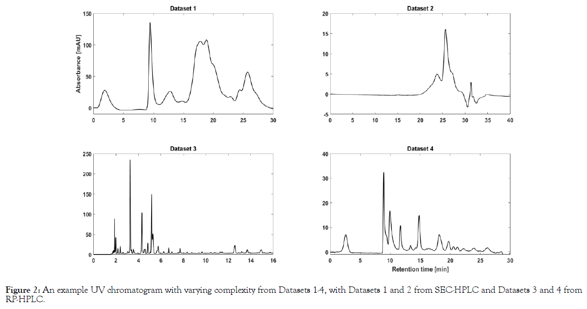
Figure 2: An example UV chromatogram with varying complexity from Datasets 1-4, with Datasets 1 and 2 from SEC-HPLC and Datasets 3 and 4 from RP-HPLC.
Reference spectrum selection
The reference spectrum is usually selected based on a priori knowledge of the dataset. The reference spectrum must be representative of the (most) significant peaks in a dataset, which is important for extracting process information using multivariate models. Often, the reference spectrum is either calculated by determining the mean or median of the entire dataset or by choosing the latest sample in the sequence which usually represents the highest number of peaks [20,21]. Skov et al. [10] proposed a selection criterion for identifying the reference spectrum by calculating the product of correlation coefficients between the chosen reference spectrum and each individual sample [10]. The reference spectra and the rationale for selecting them are shown in Table 2. Although, mean and median measures contain significant peak information, they can be biased towards a few peaks with high maxima. Thus, we opted for a bi-weighted mean approach, which imposes a bias-correction to avoid maximum peak intensities which influences the peak alignment procedure. The maximum of all chromatograms in the dataset captures all maximum values or significant peak information and therefore, was considered also as a reference spectrum. In total, seven different reference spectra were used for identifying the optimal reference spectrum for further peak alignment methods.
Table 2: Reference spectra and the rationale for selecting them for subsequent preprocessing.
| No. | Reference spectra | Rationale |
|---|---|---|
| 1 | Mean | renders a collective chromatogram containing all significant peaks in a dataset |
| 2 | Median | |
| 3 | Bi-weighted mean | avoids bias towards few peaks with high maxima |
| 4 | Maximum of all signals | captures maximum values of all chromatograms in a dataset |
| 5 | Maximum cumulative product of correlation coefficients | chromatogram with maximum correlation with all chromatograms in a dataset |
| 6 | First injection | represents all peaks at the beginning of the process |
| 7 | Last injection | represents all peaks at the end of the process |
Peak alignment techniques
Three different peak alignment methods were tested in this study. The main properties of the different alignment techniques are shown in Table 3.
Table 3: Properties of three different peak alignment methods used in this study.
| Peak alignment method | Target function | Correction method | Technique | Reference |
|---|---|---|---|---|
| icoshift | FFT cross correlation | Shift, Insert and Delete | Segmentation model | [13,17] |
| PAFFT | Shift | [18] | ||
| RAFFT | Segmentation model + recursive alignment | [18] |
All individual chromatograms which had buffer artefact peaks were considered as outliers and removed based on the Hotelling’s T2 statistic from the PCA models on raw chromatographic dataset prior to peak alignment procedures.
Icoshift: The icoshift algorithm was initially developed for ID NMR data [17], but it also has been used for UV-chromatographic data (e.g. [1,13]). The icoshift algorithm splits each UV chromatogram into segments and aligns these segments from the dataset to the segments in the reference spectrum by shifting the segments sideways to achieve maximum cross-correlation. It is driven by a FFT engine for simultaneous alignment and has been shown to outperform warping algorithms (e.g. COW; [13]). The main advantage of icoshift is its shifting procedure where the number of shifts of a particular segment can be determined either by the algorithm automatically or user-defined. In common warping algorithms, the search for the shift parameter is tedious as it is powered by dynamic programming (e.g. dynamic time warping (DTW); [20]). Some other advantages of the algorithm include high computational power, user-defined segments and option to fill in missing values (e.g. through interpolation) [17]. The algorithm is available from [22].
In this study, the number of segments was set between 1 (indicating the entire chromatogram of a sample as a segment), and the total number of data points in the datasets (eg. 4799 segments for Dataset 3). The maximum number of shifts allowed was not fixed and the algorithm was allowed to shift until it found the best fit. The chosen values for the different meta variables for icoshift are shown in the supplementary information (Table S1). Missing parts on segment edges were replaced by repeating the value of the segment edge.
Pafft: Similar to icoshift, the PAFFT algorithm also corrects misalignments by shifting the segments to achieve highest correlation. The optimal shift size is determined by sliding the segment of a sample over the corresponding segment in the reference spectrum to achieve maximum correlation. PAFFT does not allow addition of missing values with zeros or interpolations, therefore possible endpoint contamination (by addition of interpolated values) in the chosen segments may occur. On the other hand, since no extra data points are added to the UV chromatographic data, no artifacts are generated. Additionally, PAFFT provides an option to limit the number of shifts of a particular segment. PAFFT also uses the FFT engine for peak alignment. Since two metaparameters need to be defined, we used a simple two factorial screening design for exploring the optimal meta-parameter combinations. The number of segments were chosen between 1 (corresponding to all data points in each chromatogram) and 1/16 of the chromatogram length (where the entire chromatogram is split into 16 parts, with each segment containing different data points in accordance with the dataset). The number of times the chromatograms were split (16) was chosen arbitrarily and can be changed. The number of shifts allowed by the PAFFT is dependent on the complexity of the dataset. In other words, it depends on the peak properties such as retention time and peak width in the dataset, therefore we assumed a maximum shift corresponding to 1 min in the retention time. Five combinations of shifts and segments based on the experimental design were chosen for the PAFFT algorithm and are shown in Table S1. The algorithm for PAFFT can be downloaded from [23].
Rafft: RAFFT is an extensively used peak alignment method which also uses FFT cross correlation for peak alignment [16,18]. In contrast to PAFFT, the RAFFT algorithm splits the entire spectrum into smaller segments for identifying the highest correlation. The maximum number of shifts allowed for each segment is specified by the user. At the beginning of the alignment procedure, the bigger segment is selected for alignment and this segment is gradually broken down to smaller segments until either the highest correlation is achieved or the maximum number of allowed shifts is reached. RAFFT has also been shown to be faster in comparison to other warping algorithms [16]. In this study, the maximum number of shifts allowed was fixed based on the retention time as in PAFFT. We assumed that the segment, comprising of a few peaks, should not shift more than 1 min of the retention time. Therefore, we chose fixed values with 61, 121, 181, 241 and 301 shifts, corresponding to 0.2, 0.4, 0.6, 0.8 and 1 min in retention time. The algorithm for RAFFT can be downloaded [23].
Evaluation criteria
Correlation analysis: Correlation of the aligned samples from each peak alignment method with the chosen reference spectrum renders similarity measures. If all peaks in the sample dataset are aligned precisely to the reference spectrum, we obtain a correlation value of 1. However, this measure is only a rough estimate of the alignment procedure and depends entirely on the reference spectrum selection.
Explained variance: The explained variance measure calculated from the PCA model can be used to evaluate the performance of the alignment method. Perfectly aligned chromatograms have a higher variance explained in the first principal components in comparison to misaligned data. Therefore, the sum of the explained variance of the first principal component(s) was calculated for all aligned datasets by establishing PCA models on all datasets. The explained variance in combination with the correlation analysis indicate the optimal setting for a given peak alignment method.
Peak factor: Skov et al. proposed the peak factor as a measure for analyzing the performance of peak alignment techniques [10]. The peak factor measures absolute changes in the spectroscopic data due to peak alignment procedures. This is relevant since the alignment technique must not modify the actual data since any changes affect the subsequent multivariate models. The peak factor is calculated by comparing the Euclidian length (norm) of a UV chromatogram before and after alignment. For warping algorithms such as DTW, peaks from the original data have been reported to be distorted [14]. However, if there is no change in the peak shape, the peak factor has a value of 1.
Computational time: Although this measure may not be relevant for the chosen peak alignment methods used in this study, owing to their fast computations, we included this measure for applicability. Chromatographic and spectroscopic data have been successfully used for bioprocess monitoring [24-26], which necessitates fast preprocessing techniques to be on par with bioprocess dynamics [27]. Warping algorithms often have very high computational times [28]. Initially, we considered including dynamic multi-way warping (DMW) as a peak alignment method in this study. However, DMW rendered a 1,000-fold higher computational time (data not shown) than icoshift, PAFFT and RAFFT and hence was not included. However, it is practical for the user to have an overview of time invested for a particular peak alignment method. Therefore, we calculated the computational time for the chosen peak alignment procedures. We performed all analyses in a stand-alone PC with Intel i5-3330 @ 3.00 GHz processor and 8 GB RAM.
Visualization: Visual inspection of datasets renders better understanding of peak alignment methods and contributes to further improvement of the alignment procedure by optimization of metaparameters. Heat maps were used in this study for visualizing the UV chromatographic data based on their intensities. Strong misalignments can be easily identified using heat maps. For ease of visualization, 2D plots of the original and best alignment were generated to give the user a clear overview of the alignment procedure.
Multivariate models
As an application example, PCA models were developed on the original (misaligned) and the 'best' aligned datasets. In general, the PCA models are used to realize the impact of different peak alignment techniques on chemometric models. In short, PCA is an exploratory technique which decomposes the entire chromatographic dataset to a few latent principal components. Each sample is represented as a score and is projected across different principal components based on their similarities or differences. The resulting score plots from the PCA model can be used to identify possible groupings or similarities between samples in the UV chromatographic data.
Software
All data analyses were done using MATLAB R2016a (Mathworks, US). The PCA models were established in SIMCA v13.0 (Umetrics, Sweden).
Results and Discussion
In this study we developed a methodology to screen for metaparameters and to choose a peak alignment technique based on different evaluation criteria such as correlation analysis, peak factor and computational time. Four UV chromatographic datasets with varying number of samples, complexity and data volume were analyzed in this study to show the generic applicability of our workflow.
Reference spectrum selection
Seven reference spectra were generated and correlated to each UV chromatogram from all datasets. The correlation coefficients from all datasets and their respective reference spectrum are shown as boxplots in Figure 3. The line inside the box indicates the absolute correlation of the chosen reference spectrum to all four datasets.
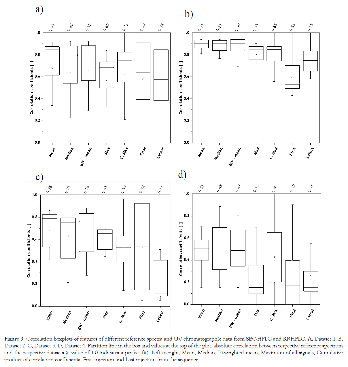
Figure 3: Correlation boxplots of features of different reference spectra and UV chromatographic data from SEC-HPLC and RP-HPLC. A, Dataset 1, B, Dataset 2, C, Dataset 3, D, Dataset 4. Partition line in the box and values at the top of the plot, absolute correlation between respective reference spectrum and the respective datasets (a value of 1.0 indicates a perfect fit). Left to right, Mean, Median, Bi-weighted mean, Maximum of all signals, Cumulative product of correlation coefficients, First injection and Last injection from the sequence.
It is interesting to note that the first and last injections from all datasets cannot be used as reference spectrum. In Datasets 1 and 2, it is clear that the first and the last injections were not representative of all peak information. Similarly, the peak information in the first and last injections represent different vitamin compositions in Dataset 3 and metabolite profiles in Dataset 4 and render the least correlation. This can be explained with the changes in analyte concentrations over process time, which indicates release (appearance of new peaks) and/or utilization (disappearance of existing peaks) over time. Since the reference spectrum calculated with the arithmetic mean of UV chromatograms, of all samples from Datasets 1-4, rendered the highest correlation, it was chosen as the optimal reference spectrum.
Evaluation criteria
Correlation analysis: Three peak alignment methods were chosen based on their FFT cross correlation for high throughput analysis and less complexity in comparison to warping algorithms. Peak alignment was done using the chosen reference spectrum from respective datasets and correlation analysis was done between the reference spectrum and aligned datasets. For each peak alignment method five different meta-parameter constraints were used. The results from the correlation analysis for all four Datasets are shown in Figure 4.
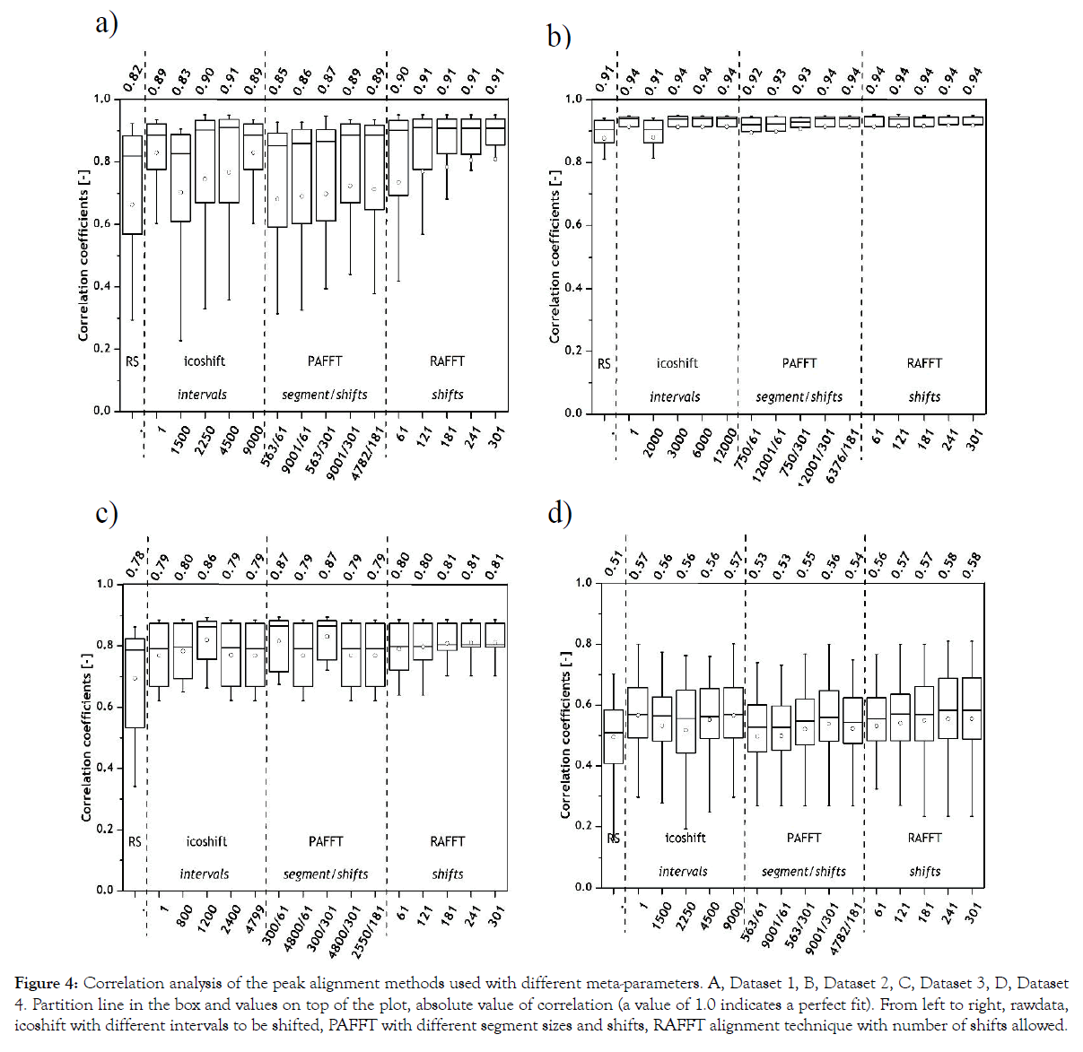
Figure 4: Correlation analysis of the peak alignment methods used with different meta-parameters. A, Dataset 1, B, Dataset 2, C, Dataset 3, D, Dataset 4. Partition line in the box and values on top of the plot, absolute value of correlation (a value of 1.0 indicates a perfect fit). From left to right, rawdata, icoshift with different intervals to be shifted, PAFFT with different segment sizes and shifts, RAFFT alignment technique with number of shifts allowed.
All the chosen methods with the chosen meta-parameters achieved high correlations above 0.83 for Dataset 1 and 0.91 for Dataset 2. Nevertheless, the RAFFT algorithm performed marginally better for both datasets, namely 0.91 was achieved for Dataset 1 and 0.94 for Dataset 2 were achieved as maximum correlation results. In Dataset 1, it is interesting to note that the RAFFT algorithm has overall lower standard deviations (as indicated with the error bars) in comparison to icoshift or PAFFT algorithms. This can be explained by complete shifts of the chromatogram in the RAFFT algorithm rather than dividing the chromatographic data into segments as in icoshift and PAFFT algorithms.
For Dataset 3 (Figure 4), the correlation coefficients of the selected reference spectrum and icoshift increased with higher intervals to be shifted, but started to decline after 1200 intervals. This indicates that the optimum intervals to be shifted using icoshift algorithm should be close to 1200 intervals. Interestingly, with PAFFT algorithm we can see a clear trend between the correlation values and the number of segments. The lower the number of segments, the higher the correlation. The RAFFT algorithm performed consistently irrespective of the number of shifts used. With Dataset 4, all peak alignment algorithms performed consistently with marginal differences within each alignment. RAFFT algorithm portrayed highest correlation in Dataset 4.
Between the two datasets from SEC-HPLC, Dataset 2 with lower number of samples rendered higher correlation and in comparison between the two datasets from RP-HPLC, Dataset 3 in general offered a higher correlation to the chosen reference spectrum. This can be explained by the differences in the number of samples considered, for example 16 samples for Dataset 3 and 51 samples for Dataset 4. Higher sample numbers leads to a wide spread of metabolite profiles from four different bioprocesses, whereas the samples from Dataset 3 comprise of almost the same vitamins.
In general, Datasets 1 and 2 achieved higher correlation results in comparison with Datasets 3 and 4. As explained earlier, RP-HPLC datasets have a complex data structure in comparison to SEC-HPLC datasets which hamper the peak alignment procedure. Summarizing the results from the correlation analysis, RAFFT algorithm with 121- 301 shifts rendered similar results (0.91) for Dataset 1, whereas icoshift, PAFFT and RAFFT rendered at least one maximum correlation with their respective settings for Dataset 2. Only with the correlation analysis, it is hard to conclude which of the alignment techniques worked best for Dataset 2. For Dataset 3, icoshift with 1200 intervals, PAFFT with 300 segments with varying shifts, RAFFT with 241 shifts rendered the highest correlation and for Dataset 4, icoshift with 1 interval or the entire chromatogram, PAFFT with 9001 segments and 301 shifts and RAFFT also with 301 shifts rendered the highest correlation.
Explained variance: The explained variance was calculated using a PCA model on the dataset and used to indicate the degree of alignment. The explained variance from the principal components for all alignment methods and their chosen meta-parameters are shown in Figure 5.
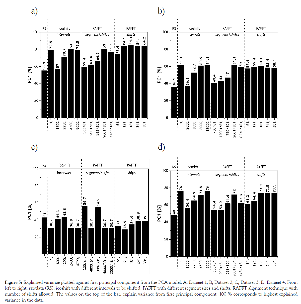
Figure 5: Explained variance plotted against first principal component from the PCA model. A, Dataset 1, B, Dataset 2, C, Dataset 3, D, Dataset 4. From left to right, rawdata (RS), icoshift with different intervals to be shifted, PAFFT with different segment sizes and shifts, RAFFT alignment technique with number of shifts allowed. The values on the top of the bar, explain variance from first principal component. 100 % corresponds to highest explained variance in the data.
Aligned chromatograms explain higher variance in the first PC from a PCA model, therefore, the higher the explained variance the better is the alignment of the dataset. For Dataset 1, the results from the explained variance are in agreement with the results achieved in correlation analysis. The RAFFT algorithm between 121-301 shifts rendered the highest explained variance for Dataset 1. It is more interesting to note in Dataset 2, the peak alignment procedure with different meta-parameters resulted in similar trend for both explained variance (> 57%) and correlation analysis (0.94). Based on the results from Dataset 2, we can clearly see icoshift algorithm 1 and 12000 intervals resulted in the highest explained variance (61.1%).
Results from the PCA models of Dataset 3 indicate that the first principal component in icoshift with 1200 segments explained 44%, PAFFT with 300 segments and 61 shifts explained 57% and RAFFT with 241 shifts explained 39%. These results are in agreement with the results from the correlation analysis. For Dataset 4, icoshift with 1 interval, PAFFT with 9001 segments and 301 shifts and RAFFT with 181 shifts indicated highest explained variances in the PCA models. Correlation analysis with Dataset 4 and RAFFT algorithm indicated 301 to render the highest correlation. However, explained variance indicates 181 shifts with RAFFT algorithm to be optimal, although 301 shifts (from correlation analysis) also has marginally the same value. Nevertheless, icoshift rendered better alignment in comparison with the other two algorithms for Dataset 4.
It is interesting to note, the higher the number of samples considered in the PCA model, the higher the average explained variance achieved. Summarizing, we chose 181 shifts for Dataset 1 since it rendered a marginally higher explained variance, whereas icoshift with 1 interval was chosen for Dataset 2. PAFFT algorithm explained the highest variance (~57%) indicating better peak alignment performance in comparison to icoshift and RAFFT algorithms for Dataset 3. As for Dataset 4, icoshift with 1 interval considering the whole chromatogram gave the highest explained variance.
Peak factor: The peak factor indicates net changes in the aligned chromatograms in comparison to the original chromatogram. The optimal peak value is ‘1’ corresponding to ‘no change’. The peak factors for almost all meta-parameter settings and peak alignment methods for Dataset 1 were higher than 0.96 (icoshift: 1500 intervals). This could be due to endpoint contaminations. For Dataset 2, all peak alignment methods resulted in a peak factor of 1, indicating no loss of information or distortion of peaks. The peak factor for Datasets 3 and 4 were higher than 0.97, which indicates that the used peak alignment methods did not alter the chromatographic information significantly (less than 3%). As mentioned earlier, peak shapes are altered mainly when warping or interpolation functions are integrated into the peak alignment procedure. However, for shift-based algorithms employed in this study little to no peak distortion is to be expected.
Computational time: The computational time was calculated to analyze the time taken for a peak alignment method to render aligned chromatograms for all datasets. For clarity, icoshift with different intervals to be shifted was analyzed in one block and, the computational time for all five settings, sixteen samples and 4,800 data points in each chromatogram for Dataset 3 was calculated for the block. The computation time taken for alignment of the entire icoshift block in Dataset 1 was 1.85 s, for the PAFFT block it was 0.23 s and RAFFT with 0.68 s. For Dataset 2, the icoshift block took 1.46 s, the PAFFT algorithm 0.18 s and RAFFT algorithm with 0.40 s. Dataset 3 with the entire icoshift block took 1.28 s, for the PAFFT block it was 0.13 s and RAFFT with 0.23 s. As for Dataset 4, icoshift algorithm took 4.47 s, PAFFT took 0.48 s and RAFFT with 1.17 s for 51 samples with 9001 data points. Comparing all four datasets, the increasing order of computation time can be clearly seen with the increase in the number of samples. The PAFFT algorithm always rendered the minimal computational time for all the datasets considered in this study. However it has to be noted that the PAFFT algorithm performed less in terms of correlation and explained variance with comparison to other peak alignment procedures. Warping algorithms are usually 100-folds higher in computational time in comparison to the FFT correlation methods used in this study [10]. Overall, all algorithms used in this study took less than 5 seconds for peak alignment procedure.
Visualization: Heat maps or 2D plots can be used to visualize the alignment results. In heat maps, the intensities of the significant peaks are highlighted and possible misalignments are identified. Furthermore, any improvement on a peak alignment method based on a different set of meta-parameters can be directly seen. The results from the heat map and 2D plots of the chosen methods, from Datasets 1-4, showing the unaligned dataset and best alignments achieved are shown in Figure S1. The heat maps from the original and best aligned datasets clearly highlights the misalignments in the raw dataset and alignment efficiency of the algorithm. The 2D plots shows the efficiency of the alignment procedure, where one can clearly see the improvement in peak alignment. Finally, any outliers in the UV chromatographic data can be easily identified (e.g. buffer peaks) by visualizing peak distortions using heat maps.
From all these results, we can see that the correlation analysis and explained variance rendered similar indications to peak alignment performance for the chosen meta-parameters. Peak factor resulted in similar results and indicated no interference in the peak properties, thereby no loss in information. The correlation analysis and explained variance indicated RAFFT with 181 shifts for Dataset 1 and icoshift with 1 interval for Dataset 2. For Dataset 3, PAFFT algorithm with 300 segment size and 61 shifts performed better than all other peak alignment algorithms used in this study, whereas for Dataset 4, icoshift algorithm with 1 interval considering the whole chromatogram outperformed all other algorithms. It is clear that no golden standard of preprocessing technique is available globally for all datasets. However, such a generic strategy must be used to screen for different preprocessing techniques to avoid misleading multivariate models. In order to describe deviations in modeling results, we chose the original datasets, the best aligned datasets and the worst aligned datasets for establishing multivariate models.
Multivariate models
PCA models were established on the 'best' alignments and worst alignments achieved from the peak alignment technique which was identified from all datasets. PCA models render different model variables such as scores and loadings which can be used to extract relevant information from the input datasets. In PCA, the closer the scores are to each other the more similar they are, with respect to the principal components. We analyzed the performance of the peak alignment technique based on the trends in score plots from the PCA models. The score scatter plots from the PCA model from Datasets 1-4 are shown in Figure 6A-6D.
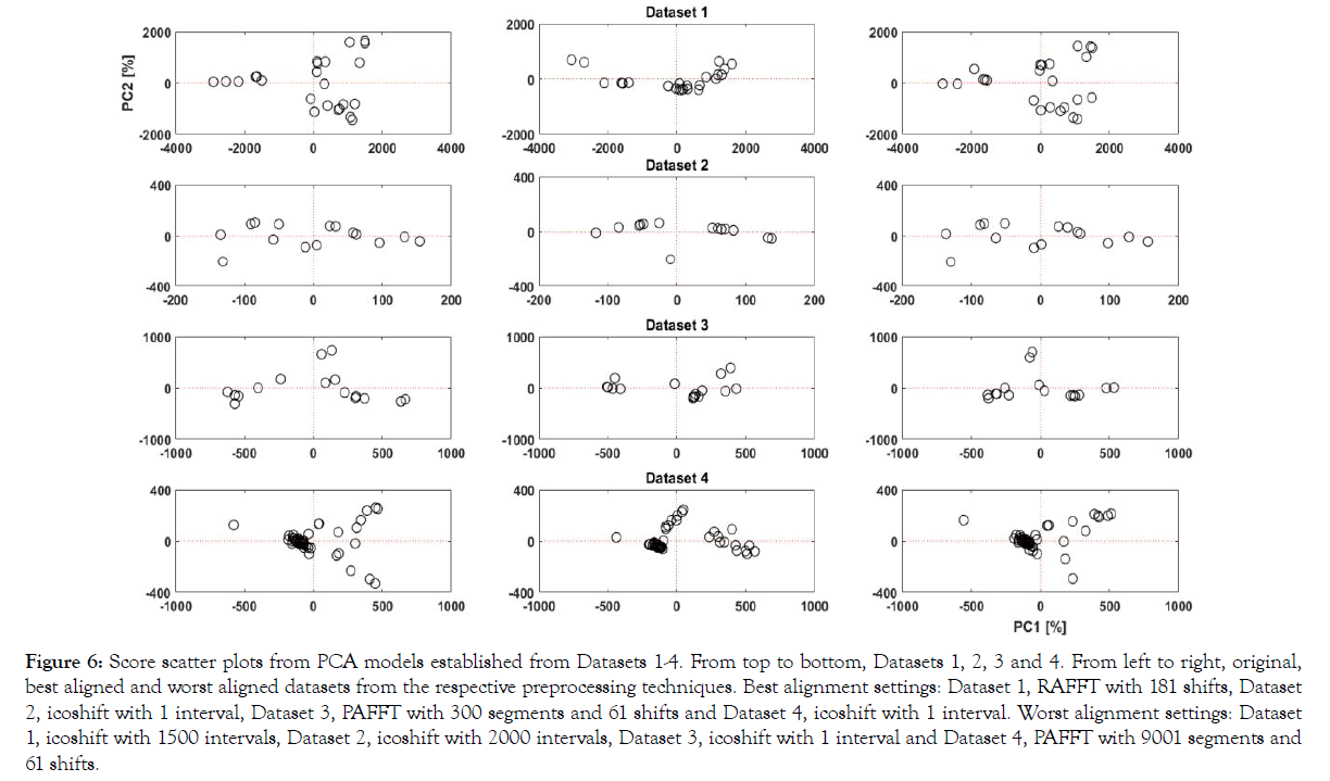
Figure 6: Score scatter plots from PCA models established from Datasets 1-4. From top to bottom, Datasets 1, 2, 3 and 4. From left to right, original, best aligned and worst aligned datasets from the respective preprocessing techniques. Best alignment settings: Dataset 1, RAFFT with 181 shifts, Dataset 2, icoshift with 1 interval, Dataset 3, PAFFT with 300 segments and 61 shifts and Dataset 4, icoshift with 1 interval. Worst alignment settings: Dataset 1, icoshift with 1500 intervals, Dataset 2, icoshift with 2000 intervals, Dataset 3, icoshift with 1 interval and Dataset 4, PAFFT with 9001 segments and 61 shifts.
In Figure 6, the score plot of the original data shows a wide spread of scores each representing a UV chromatogram. In the best alignment, we can see a compact trend where samples similar to each other are projected closer. This is further highlighted with the score plot from the worst alignment, where the scores are even more scattered than the scores from original data showing strong dissimilarities. We can see a clear improvement, between the original dataset and the best alignment with respect to clustering in the score plot, highlighting the peak alignment performance. Similarly, we can clearly see similarities between the original and worst aligned datasets for all datasets. In Figure 6, original and worst datasets yield almost identical results as suggested from the very similar results in the evaluation criteria (i.e. 36.1%, 36.8% explained variance for original and worst aligned datasets). It is interesting to note that in Dataset 4, the best and worst alignment was achieved with the same algorithm (icoshift) with different metaparameters (intervals). This further highlights the significance of metaparameters in peak alignment procedures and the subsequent data driven models.
Conclusion
UV chromatographic data are prone to shifts along the retention time, which requires preprocessing prior to establishing multivariate models. In this study, we established a generic strategy for screening and validating different preprocessing techniques for UV chromatographic data. We chose different peak alignment techniques with different meta-parameters to evaluate their performance on four datasets. We analyzed the performance using different statistical tools to identify the optimal peak alignment technique and its meta-parameter ranges. The evaluation from statistical tools illustrated that peak alignment techniques, even though similar in correction methods and target functions, can render different results. The complexity and the sample numbers of each dataset also have an impact on the peak alignment procedure. Therefore, it is safe to hypothesize that the performance of the peak alignment technique is dependent on the initial, raw dataset and no global standard exists for all datasets. The impact of the metaparameters of the chosen peak alignment technique affects the model results, which can be highlighted with the score scatter plots from the PCA models. Summarizing, the proposed methodology was used to choose the reference spectrum, screen for meta-parameter ranges and validate the results using data driven models. The generic methodology can be used for different chromatographic datasets and has a modularsetup which allows incorporation of any peak alignment technique and any statistical tool as evaluation criterion. We envision the proposed workflow also for spectroscopic data which is usually hampered with peak and baseline shifts.
Conflict of Interests
The authors declare that they have no competing interests.
Acknowledgements
The authors thank Britta Eggenreich, Alexandra Hofer and David Wurm (TU Wien, Austria) for their kind provision of chromatographic datasets and process specific information.
Author Contributions
Vignesh Rajamanickam and Oliver Spadiut initiated, designed and planned the study. Vignesh Rajamanickam established the workflow, executed the models and wrote the manuscript. Oliver Spadiut and Christoph Herwig supervised the work.
Funding
This research did not receive any specific grant from funding agencies in the public, commercial, or not-for-profit sectors.
REFERENCES
- Rajamanickam V, Wurm D, Slouka C, Herwig C, Spadiut O. A novel toolbox for E. coli lysis monitoring. Anal Bioanal Chem. 2016;409:1-5.
- Rathore AS. Follow-on protein products: scientific issues, developments and challenges. Trends Biotechnol. 2009;27:698-705.
- Wang J, Lam H. Graph-based peak alignment algorithms for multiple liquid chromatography-mass spectrometry datasets. Bioinformatics. 2013;29:2469-2476.
- Watrous JD, Henglin M, Claggett B, Lehmann KA, Larson MG, Cheng S, et al. Visualization, Quantification, and Alignment of Spectral Drift in Population Scale Untargeted Metabolomics Data. Anal Chem. 2017;89:1399-1404.
- Malherbe CJ, de Beer D, Joubert E. Development of on-line high performance liquid chromatography (HPLC)-biochemical detection methods as tools in the identification of bioactives. Int J Mol Sci. 2012;13:3101-3133.
- Jensen TB, Marley PD. Development of an assay for histamine using automated high-performance liquid chromatography with electrochemical detection. J Chromatogr B Biomed Appl. 1995;670:199-207.
- Schmid J, Beschke K. The use of high-performance liquid chromatography in biochemical and medical analyses. Arzneimittelforschung. 1978;28:1969-1974.
- Smilde AK, Bro R, Geladi P. Multi-way analysis Applications in the chemical sciences, John Wiley & Sons Ltd., Chichester, England. 2004.
- de Juan A, Tauler R. Comparison of three-way resolution methods for non-trilinear chemical data sets. J Chemom. 2001;15:749-771.
- Skov T, van den Berg F, Tomasi G, Bro R. Automated alignment of chromatographic data. J Chemom. 2007;20:484-497.
- Nielsen NPV, Carstensen JM, Smedsgaard J. Aligning of single and multiple wavelength chromatographic profiles for chemometric data analysis using correlation optimized warping. J Chromatogr A. 1998;805:17-35.
- Forshed J, Schuppe-Koistinen I, Jacobsson SP. Peak alignment of NMR signals by means of a genetic algorithm. Anal Chim Acta. 2003;487:189-199.
- Tomasi G, Savorani F, Engelsen SB. Icoshift: An effective tool for the alignment of chromatographic data. J Chromatogr A. 2011;1218:7832-7840.
- Vu TN, Laukens K. Getting your peaks in line: a review of alignment methods for NMR spectral data. Metabolites. 2013;3:259-276.
- Giskeødegård GF, Bloemberg TG, Postma G, Sitter B, Tessem MB, Gribbestad IS, et al. Alignment of high resolution magic angle spinning magnetic resonance spectra using warping methods. Anal Chim Acta. 2010;683:1-11.
- He QP, Wang J. Comparison of a new spectrum alignment algorithm with other methods. Am Control Conf. 2010:1260-1265.
- Savorani F, Tomasi G, Engelsen SB. Icoshift: A versatile tool for the rapid alignment of 1D {NMR} spectra. J Magn Reson. 2010;202:190-202.
- Wong JW, Durante C, Cartwright HM. Application of Fast Fourier Transform Cross-Correlation for the Alignment of Large Chromatographic and Spectral Datasets. Anal Chem. 2005;77:5655-5661.
- Hofer A, Herwig C. Quantitative determination of nine water-soluble vitamins in the complex matrix of corn steep liquor for raw material quality assessment. J Chem Technol Biotechnol. 2017;92:2106-2113.
- Tomasi G, van den Berg F, Andersson C. Correlation optimized warping and dynamic time warping as preprocessing methods for chromatographic data. J Chemom. 2004;18:231-241.
- Pravdova V, Walczak B, Massart DL. A comparison of two algorithms for warping of analytical signals. Anal Chim Acta. 2002;456:77-92.
- Tomasi G, Savorani F. Icoshift-An ultra-rapid and versatile tool for the alignment of spectral datasets. 2017.
- UNSW Medicine. SpecAlign-processing and alignment of spectral datasets. 2017.
- Vaidyanathan S, Arnold SA, Matheson L, Mohan P, McNeil B, Harvey LM. Assessment of near-infrared spectral information for rapid monitoring of bioprocess quality. Biotechnol Bioeng. 2001;74:376-388.
- Clavaud M, Roggo Y, Von Daeniken R, Liebler A, Schwabe JO. Chemometrics and in-line near infrared spectroscopic monitoring of a biopharmaceutical Chinese hamster ovary cell culture: prediction of multiple cultivation variables. Talanta. 2013;111:28-38.
- Wu Y, Jin Y, Li Y, Sun D, Liu X, Chen Y. NIR spectroscopy as a process analytical technology (PAT) tool for on-line and real-time monitoring of an extraction process. Vib Spectrosc. 2012;58:109-118.
- Rathore AS, Bhambure R, Ghare V. Process analytical technology (PAT) for biopharmaceutical products. Anal Bioanal Chem. 2010;398:137-154.
- Zhou F, De La Torre F. Generalized time warping for multi-modal alignment of human motion, Proc. IEEE Comput. Soc. Conf. Comput. Vis. Pattern Recognit. 2012:1282-1289.
Citation: Rajamanickam V, Herwig C, Spadiut O (2019) A Generic Workflow for Bioprocess Analytical Data: Screening Alignment Techniques and Analyzing their Effects on Multivariate Modeling. Biochem Anal Biochem 8:373. doi: 10.35248/2161-1009.19.8.373.
Copyright: © 2019 Rajamanickam V, et al. This is an open-access article distributed under the terms of the Creative Commons Attribution License, which permits unrestricted use, distribution, and reproduction in any medium, provided the original author and source are credited.
